Visualization & Style Transfer

Shan-Hung Wu & DataLab
Fall 2024

This tutorial is going to show how to load and use a pretrained model from tensorflow library and discusses some techniques to visualize what the networks represent in the selected layers. In addition, we will introduce an interesting work called neural style transfer, using deep learning to compose one image in the style of another image.

Import and configure modules

import tensorflow as tf
import numpy as np
import time
import functools
import IPython.display as display
from pathlib import Path
import random
from PIL import Image
from matplotlib import pyplot
import matplotlib.pyplot as plt
import matplotlib as mpl
import os

mpl.rcParams['figure.figsize'] = (12,12)
mpl.rcParams['axes.grid'] = False

gpus = tf.config.experimental.list_physical_devices('GPU')
if gpus:
    try:
        # Restrict TensorFlow to only use the fourth GPU
        tf.config.experimental.set_visible_devices(gpus[0], 'GPU')

        # Currently, memory growth needs to be the same across GPUs
        for gpu in gpus:
            tf.config.experimental.set_memory_growth(gpu, True)
        logical_gpus = tf.config.experimental.list_logical_devices('GPU')
        print(len(gpus), "Physical GPUs,", len(logical_gpus), "Logical GPUs")
    except RuntimeError as e:
        # Memory growth must be set before GPUs have been initialized
        print(e)

2 Physical GPUs, 1 Logical GPUs

Visualize Convolutional Neural Networks

Visualize the input

Define a function to load an image and limit its maximum dimension to 512 pixels.

def load_img(path_to_img):
    max_dim = 512
    img = tf.io.read_file(path_to_img)
    img = tf.image.decode_image(img, channels=3)
    img = tf.image.convert_image_dtype(img, tf.float32)

    shape = tf.cast(tf.shape(img)[:-1], tf.float32)
    long_dim = max(shape)
    scale = max_dim / long_dim

    new_shape = tf.cast(shape * scale, tf.int32)

    img = tf.image.resize(img, new_shape)
    # in order to use CNN, add one additional dimension 
    # to the original image
    # img shape: [height, width, channel] -> [batch_size, height, width, channel]
    img = img[tf.newaxis, :]
    
    return img

Create a simple function to display an image:

def imshow(image, title=None):
    if len(image.shape) > 3:
        image = tf.squeeze(image, axis=0)

    plt.imshow(image)
    if title:
        plt.title(title)

content_path = './dataset/content_nthu.jpg'
content_image = load_img(content_path)
print('Image shape:', content_image.shape)
imshow(content_image, 'Content Image')

Image shape: (1, 341, 512, 3)

Load a pretrained network (VGG19)

We are going to visualize one of most remarkable neural networks, VGG19, which is introduced from this paper, pretrained on ImageNet. VGG19 is known for its simplicity, using only 3×3 convolutional layers stacked on top of each other in increasing depth. The "19" in its name stands for the number of layers in the network. ImageNet is a large dataset used in ImageNet Large Scale Visual Recognition Challenge(ILSVRC). The training dataset contains around 1.2 million images composed of 1000 different types of objects. The pretrained network learned how to create useful representations of the data to differentiate between different classes.

Pretrained network is useful and conveninent for several further usage, such as style transfer, transfer learning, fine-tuning, and so on. Generally, using pretrained network can save a lot of time and also easier to train a model on more complex dataset or small dataset.

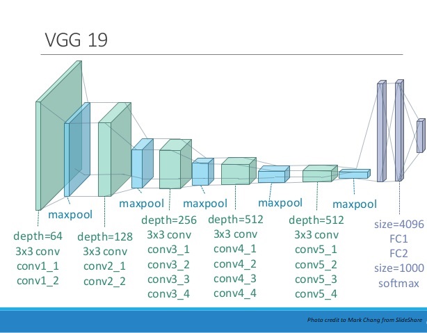
Load a VGG19 and test run it on our image to ensure it's used correctly. The output of VGG19 is the probabilities corresponding to 1000 categories.

x = tf.keras.applications.vgg19.preprocess_input(content_image*255)
x = tf.image.resize(x, (224, 224))

# load pretrained network(VGG19)
vgg = tf.keras.applications.VGG19(include_top=True, weights='imagenet')
prediction_probabilities = vgg(x)
prediction_probabilities.shape

TensorShape([1, 1000])

Obtain the top 5 predicted categories of the input image.

predicted_top_5 = tf.keras.applications.vgg19.decode_predictions(prediction_probabilities.numpy())[0]
[(class_name, prob) for (number, class_name, prob) in predicted_top_5]

[('library', 0.5540086),
 ('bookshop', 0.097569965),
 ('bell_cote', 0.06389093),
 ('church', 0.048398577),
 ('cinema', 0.030339612)]

Let's try to first print out the detailed structure of VGG19. vgg.summary() shows the name, output shape and the number of parameters of each layer.

vgg.summary()

Model: "vgg19"
_________________________________________________________________
 Layer (type)                Output Shape              Param #   
=================================================================
 input_2 (InputLayer)        [(None, 224, 224, 3)]     0         
                                                                 
 block1_conv1 (Conv2D)       (None, 224, 224, 64)      1792      
                                                                 
 block1_conv2 (Conv2D)       (None, 224, 224, 64)      36928     
                                                                 
 block1_pool (MaxPooling2D)  (None, 112, 112, 64)      0         
                                                                 
 block2_conv1 (Conv2D)       (None, 112, 112, 128)     73856     
                                                                 
 block2_conv2 (Conv2D)       (None, 112, 112, 128)     147584    
                                                                 
 block2_pool (MaxPooling2D)  (None, 56, 56, 128)       0         
                                                                 
 block3_conv1 (Conv2D)       (None, 56, 56, 256)       295168    
                                                                 
 block3_conv2 (Conv2D)       (None, 56, 56, 256)       590080    
                                                                 
 block3_conv3 (Conv2D)       (None, 56, 56, 256)       590080    
                                                                 
 block3_conv4 (Conv2D)       (None, 56, 56, 256)       590080    
                                                                 
 block3_pool (MaxPooling2D)  (None, 28, 28, 256)       0         
                                                                 
 block4_conv1 (Conv2D)       (None, 28, 28, 512)       1180160   
                                                                 
 block4_conv2 (Conv2D)       (None, 28, 28, 512)       2359808   
                                                                 
 block4_conv3 (Conv2D)       (None, 28, 28, 512)       2359808   
                                                                 
 block4_conv4 (Conv2D)       (None, 28, 28, 512)       2359808   
                                                                 
 block4_pool (MaxPooling2D)  (None, 14, 14, 512)       0         
                                                                 
 block5_conv1 (Conv2D)       (None, 14, 14, 512)       2359808   
                                                                 
 block5_conv2 (Conv2D)       (None, 14, 14, 512)       2359808   
                                                                 
 block5_conv3 (Conv2D)       (None, 14, 14, 512)       2359808   
                                                                 
 block5_conv4 (Conv2D)       (None, 14, 14, 512)       2359808   
                                                                 
 block5_pool (MaxPooling2D)  (None, 7, 7, 512)         0         
                                                                 
 flatten (Flatten)           (None, 25088)             0         
                                                                 
 fc1 (Dense)                 (None, 4096)              102764544 
                                                                 
 fc2 (Dense)                 (None, 4096)              16781312  
                                                                 
 predictions (Dense)         (None, 1000)              4097000   
                                                                 
=================================================================
Total params: 143,667,240
Trainable params: 143,667,240
Non-trainable params: 0
_________________________________________________________________

Visualize filters

Now we can visualize the weights of the convolution filters to help us understand what neural network have learned. In neural network terminology, the learned filters are simply weights, yet because of the specialized two-dimensional structure of the filters, the weight values have a spatial relationship to each other and plotting each filter as a two-dimensional image is meaningful (or could be).

We can access the block of filters and the block of bias values through layer.get_weight(). In VGG19, all convolitional layers use 3x3 filters.

# summarize filter shapes
for layer in vgg.layers:
    # check for convolutional layer
    if 'conv' not in layer.name:
        continue
    # get filter weights
    filters, biases = layer.get_weights()
    print(layer.name, filters.shape)

block1_conv1 (3, 3, 3, 64)
block1_conv2 (3, 3, 64, 64)
block2_conv1 (3, 3, 64, 128)
block2_conv2 (3, 3, 128, 128)
block3_conv1 (3, 3, 128, 256)
block3_conv2 (3, 3, 256, 256)
block3_conv3 (3, 3, 256, 256)
block3_conv4 (3, 3, 256, 256)
block4_conv1 (3, 3, 256, 512)
block4_conv2 (3, 3, 512, 512)
block4_conv3 (3, 3, 512, 512)
block4_conv4 (3, 3, 512, 512)
block5_conv1 (3, 3, 512, 512)
block5_conv2 (3, 3, 512, 512)
block5_conv3 (3, 3, 512, 512)
block5_conv4 (3, 3, 512, 512)

Let's look at every single individual filter in the first convolutional layer. We will see all 64 in the block and plot each of the three channels. It is worth to meantion that in the first convolutional layer, it has total 192 feature maps(64 filters * 3 channels). We can normalize their values to the range 0-1 to make them easy to visualize.

The dark squares indicate small or inhibitory weights and the light squares represent large or excitatory weights. Using this intuition, we can see that the filters on the first row detect a gradient from light in the top left to dark in the bottom right.

plt.figure(figsize=(16,16))

# retrieve weights from the second hidden layer
filters, biases = vgg.layers[1].get_weights()

# normalize filter values to 0-1 so we can visualize them
f_min, f_max = filters.min(), filters.max()
filters = (filters - f_min) / (f_max - f_min)

# plot first few filters
n_filters, ix = 64, 1

for i in range(n_filters):
    # get the filter
    f = filters[:, :, :, i]
    # plot each channel separately
    for j in range(3):
        # specify subplot and turn of axis
        ax = pyplot.subplot(14, 14, ix)
        ax.set_xticks([])
        ax.set_yticks([])
        # plot filter channel in grayscale
        pyplot.imshow(f[:, :, j], cmap='gray')
        ix += 1
        
# show the figure
pyplot.show()

Visualize feature maps

The activation maps, called feature maps, capture the result of applying the filters to input, such as the input image or another feature map. The idea of visualizing a feature map for a specific input image would be to understand what features of the input are detected or preserved in the feature maps. The expectation would be that the feature maps close to the input detect small or fine-grained detail, whereas feature maps close to the output of the model capture more general features.

We can see that the result of applying the filters in the first convolutional layer is a lot of versions of the input image with different features highlighted. For example, some highlight lines, other focus on the background or the foreground.

plt.figure(figsize=(16,16))

# redefine model to output right after the first hidden layer
model = tf.keras.Model(inputs=[vgg.input], outputs=vgg.layers[1].output)
model.summary()

# preprocess input
content_image = tf.keras.applications.vgg19.preprocess_input(content_image*255)
content_image = tf.image.resize(content_image, (224, 224))

# get feature map for first hidden layer
feature_maps = model.predict(content_image)

# plot all 64 maps in an 8x8 squares
square = 8
ix = 1
for _ in range(square):
    for _ in range(square):
        # specify subplot and turn of axis
        ax = pyplot.subplot(square, square, ix)
        ax.set_xticks([])
        ax.set_yticks([])
        # plot filter channel in grayscale
        pyplot.imshow(feature_maps[0, :, :, ix-1], cmap='gray')
        ix += 1
        
# show the figure
pyplot.show()

Model: "model"
_________________________________________________________________
Layer (type)                 Output Shape              Param #   
=================================================================
input_1 (InputLayer)         [(None, 224, 224, 3)]     0         
_________________________________________________________________
block1_conv1 (Conv2D)        (None, 224, 224, 64)      1792      
=================================================================
Total params: 1,792
Trainable params: 1,792
Non-trainable params: 0
_________________________________________________________________

Let's visualize the feature maps output from each block of the model. You might notice that the number of feature maps (e.g. depth or number of channels) in deeper layers is much more than 64, such as 256 or 512. Nevertheless, we can cap the number of feature maps visualized at 64 for consistency.

We can see that the feature maps closer to the input of the model capture a lot of fine detail in the image and that as we progress deeper into the model, the feature maps show less and less detail.

This pattern was to be expected, as the model abstracts the features from the image into more general concepts that can be used to make a classification. Although it is not clear from the final image that the model saw NTHU campus, we generally lose the ability to interpret these deeper feature maps.

# get feature maps for last convolutional layer in each block
ixs = [2, 5, 10, 15, 20]
outputs = [vgg.layers[i].output for i in ixs]
model = tf.keras.Model(inputs=[vgg.input], outputs=outputs)
feature_maps = model.predict(content_image)

# plot the output from each block
square = 8
for i, fmap in enumerate(feature_maps):
    # plot all 64 maps in an 8x8 squares
    ix = 1
    print(outputs[i])
    plt.figure(figsize=(16,16))
    for _ in range(square):
        for _ in range(square):
            # specify subplot and turn of axis
            ax = pyplot.subplot(square, square, ix)
            ax.set_xticks([])
            ax.set_yticks([])
            # plot filter channel in grayscale
            pyplot.imshow(fmap[0, :, :, ix-1], cmap='gray')
            ix += 1
            
    # show the figure
    pyplot.show()

Tensor("block1_conv2/Identity:0", shape=(None, 224, 224, 64), dtype=float32)

Tensor("block2_conv2/Identity:0", shape=(None, 112, 112, 128), dtype=float32)

Tensor("block3_conv4/Identity:0", shape=(None, 56, 56, 256), dtype=float32)

Tensor("block4_conv4/Identity:0", shape=(None, 28, 28, 512), dtype=float32)

Tensor("block5_conv4/Identity:0", shape=(None, 14, 14, 512), dtype=float32)

Visualize gradients

Visualizing convolutional output is a pretty useful technique for visualizing shallow convolution layers, but when we get into the deeper layers, it's hard to understand them just by just looking at the convolution output.

If we want to understand what the deeper layers are really doing, we can try to use backpropagation to show us the gradients of a particular neuron with respect to our input image. We will make a forward pass up to the layer that we are interested in, and then backpropagate to help us understand which pixels contributed the most to the activation of that layer.

We first create an operation which will find the maximum neurons among all activations in the required layer, and then calculate the gradient of that objective with respect to the input image.

def vgg_layers(layer_names):
    """ Creates a vgg model that returns a list of intermediate output values."""
    # Load our model. Load pretrained VGG, trained on imagenet data
    vgg = tf.keras.applications.VGG19(include_top=False, weights='imagenet')
    vgg.trainable = False

    outputs = [vgg.get_layer(name).output for name in layer_names]

    model = tf.keras.Model([vgg.input], outputs)
    return model

class GradientModel(tf.keras.models.Model):
    def __init__(self, layers):
        super(GradientModel, self).__init__()
        self.vgg =  vgg_layers(layers)
        self.num_style_layers = len(layers)
        self.vgg.trainable = False
        
    # return the feature map of required layer
    def call(self, inputs):
        "Expects float input in [0,1]"
        inputs = inputs*255.0
        preprocessed_input = tf.keras.applications.vgg19.preprocess_input(inputs)
        outputs = self.vgg(preprocessed_input)
        return outputs

Compute the gradient of maximum neurons among all activations in the required layer with respect to the input image.

@tf.function()
def visualize_gradient(image):
    with tf.GradientTape() as tape:
        feature = extractor(image)
        # grad = d_feature/d_image
        grad = tape.gradient(tf.reduce_max(feature, axis=3), image)
    return grad

content_image = load_img(content_path)

# activation layer
layers = ['block4_conv2']
image = tf.Variable(content_image)

extractor = GradientModel(layers)
grad = visualize_gradient(image)

# look at the range of gradients
print("shape: ", grad.numpy().shape)
print("min: ", grad.numpy().min())
print("max: ", grad.numpy().max())
print("mean: ", grad.numpy().mean())

2022-11-07 11:51:32.245482: W tensorflow/core/platform/profile_utils/cpu_utils.cc:128] Failed to get CPU frequency: 0 Hz
2022-11-07 11:51:32.249772: I tensorflow/core/grappler/optimizers/custom_graph_optimizer_registry.cc:113] Plugin optimizer for device_type GPU is enabled.

shape:  (1, 341, 512, 3)
min:  -13911.978
max:  14002.524
mean:  -18.048296

It is hard to understand the gradient in that range of values. We can normalize the gradient in a way that lets us see it more in terms of the normal range of color values. After normalizing the gradient values, let's visualize the original image and the output of the backpropagated gradient.

# normalize filter values to 0-1 so we can visualize them
g_min, g_max = grad.numpy().min(), grad.numpy().max()
filters = (grad - g_min) / (g_max - g_min)

plt.figure(figsize=(14,10))
plt.subplot(1, 2, 1)
imshow(image.read_value()[0])

plt.subplot(1, 2, 2)
imshow(filters[0])

We can also visualize the gradient of any single feature map.

@tf.function()
def visualize_gradient_single_layer(image, layer_i):
    with tf.GradientTape() as tape:
        feature = extractor(image)
        grad = tape.gradient(tf.reduce_mean(feature[:, :, :, layer_i]), image)
    return grad

plt.figure(figsize=(14,10))

grad = visualize_gradient_single_layer(image, 77)

# normalize filter values to 0-1 so we can visualize them
g_min, g_max = grad.numpy().min(), grad.numpy().max()
filters = (grad - g_min) / (g_max - g_min)

plt.figure(figsize=(14,10))
plt.subplot(1, 2, 1)
imshow(image.read_value()[0])

plt.subplot(1, 2, 2)
imshow(filters[0])

2022-11-07 11:51:39.560716: I tensorflow/core/grappler/optimizers/custom_graph_optimizer_registry.cc:113] Plugin optimizer for device_type GPU is enabled.

<Figure size 1008x720 with 0 Axes>

Guided-Backpropagation

As we can see above, the results are still hard to explain and not very satisfying. Every pixel influences the neuron via multiple hidden neurons.

Ideally, neurons act like detectors of particular image features. We are only interested in what image features the neuron detects, not in what kind of stuff it doesn’t detect. Therefore, when propagating the gradient, we set all the negative gradients to 0.

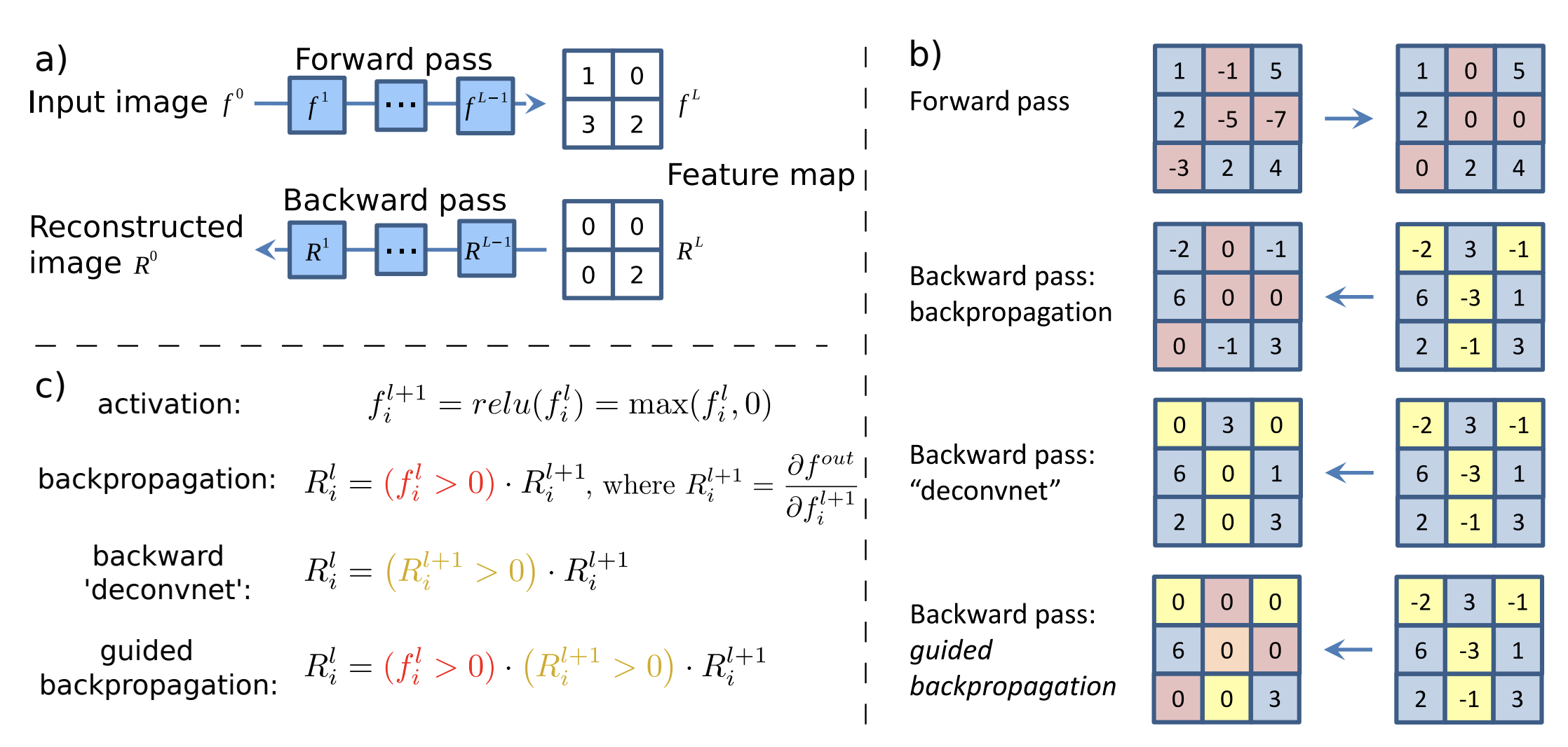
We call this method guided backpropagation, because it adds an additional guidance signal from the higher layers to usual backpropagation. This prevents backward flow of negative gradients, corresponding to the neurons which decrease the activation of the higher layer unit we aim to visualize. For more details, please refer to Striving for Simplicity: The All Convolutional Net, a nice work from J. T. Springenberg and A. Dosovitskiy et al.

from guided_backprop import GuidedBackprop

x = tf.keras.applications.vgg19.preprocess_input(content_image*255)
x = tf.image.resize(x, (224, 224))

# backprop_vgg = GuidedBackprop(model=vgg, layerName='predictions') # original
backprop_vgg = GuidedBackprop(model=vgg, layerName='block5_conv4') # use this layer instead, b/c we need to extract from vgg19.
grad = backprop_vgg.guided_backprop(x)[0].numpy()

2022-11-07 12:33:47.948977: I tensorflow/core/grappler/optimizers/custom_graph_optimizer_registry.cc:113] Plugin optimizer for device_type GPU is enabled.

# plot the original image and the three saliency map variants
plt.figure(figsize=(16, 16), facecolor='w')
plt.subplot(2, 2, 1)
plt.title('Input')
plt.imshow(tf.image.resize(content_image, (224, 224))[0])
plt.subplot(2, 2, 2)
plt.title('Abs. saliency')
plt.imshow(np.abs(grad).max(axis=-1), cmap='gray')
plt.subplot(2, 2, 3)
plt.title('Pos. saliency')
plt.imshow((np.maximum(0, grad) / grad.max()))
plt.subplot(2, 2, 4)
plt.title('Neg. saliency')
plt.imshow((np.maximum(0, -grad) / -grad.min()))
plt.show()

A Neural Algorithm of Artistic Style

Visualizing neural network gives us a better understanding of what's going in the mysterious huge network. Besides from this application, Leon Gatys and his co-authors has a very interesting work called "A Neural Algorithm of Artistic Style" that uses neural representations to separate and recombine content and style of arbitrary images, providing a neural algorithm for the creation of artistic images.

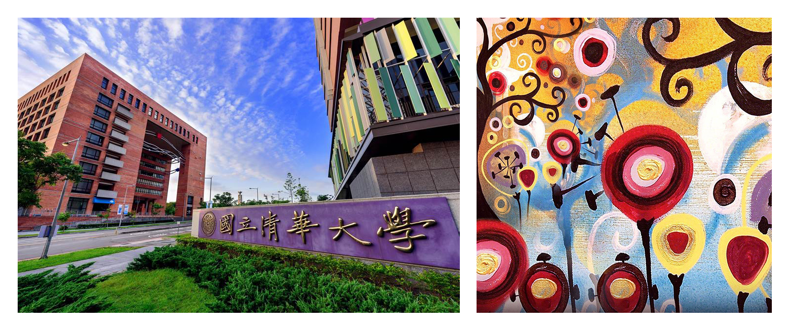
Define content and style representations

Use the intermediate layers of the model to get the content and style representations of the image. Starting from the network's input layer, the first few layers' activations represent low-level features like edges and textures. As you step through the network, the final few layers represent higher-level features—object parts like wheels or eyes. In this case, you are using the VGG19 network architecture, a pretrained image classification network. These intermediate layers are necessary to define the representation of content and style from the images. For an input image, try to match the corresponding style and content target representations at these intermediate layers.

content_path = './dataset/content_nthu.jpg'
style_path = './dataset/style_starry_night.jpg'

content_image = load_img(content_path)
style_image = load_img(style_path)

plt.figure(figsize=(14,10))
plt.subplot(1, 2, 1)
imshow(content_image, 'Content Image')

plt.subplot(1, 2, 2)
imshow(style_image, 'Style Image')

Now load a VGG19 without the classification head, and list the layer names.

vgg = tf.keras.applications.VGG19(include_top=False, weights='imagenet')

print()
for layer in vgg.layers:
    print(layer.name)

input_3
block1_conv1
block1_conv2
block1_pool
block2_conv1
block2_conv2
block2_pool
block3_conv1
block3_conv2
block3_conv3
block3_conv4
block3_pool
block4_conv1
block4_conv2
block4_conv3
block4_conv4
block4_pool
block5_conv1
block5_conv2
block5_conv3
block5_conv4
block5_pool

• Content features of the content image is calculated by feeding the content image into the neural network, and extract the activations of those content_layers.

• For style features, we extract the correlation of the features of the style-image layer-wise (gram matrix). By adding up the feature correlations of multiple layers, which corresponding to style_layers, we obtain a multi-scale representation of the input image, which captures its texture information instead of the object arrangement in the input image.

# Content layer where will pull our feature maps
content_layers = ['block5_conv2'] 

# Style layer of interest
style_layers = ['block1_conv1',
                'block2_conv1',
                'block3_conv1', 
                'block4_conv1', 
                'block5_conv1']

num_content_layers = len(content_layers)
num_style_layers = len(style_layers)

At a high level, in order for a network to perform image classification (which this network has been trained to do), it must understand the image. This requires taking the raw image as input pixels and building an internal representation that converts the raw image pixels into a complex understanding of the features present within the image.

This is also a reason why convolutional neural networks are able to generalize well: they’re able to capture the invariances and defining features within classes (e.g. cats vs. dogs) that are agnostic to background noise and other nuisances. Thus, between the raw image fed into the model and the output, in this case, the predicted label, the model serves as a complex feature extractor. By accessing intermediate layers of the model, you're able to describe the content and style of input images.

Build the model

The networks in tf.keras.applications are designed so you can easily extract the intermediate layer values using the Keras functional API.

To define a model using the functional API, specify the inputs and outputs:

model = Model(inputs, outputs)

def vgg_layers(layer_names):
    """ Creates a vgg model that returns a list of intermediate output values."""
    # Load our model. Load pretrained VGG, trained on imagenet data
    vgg = tf.keras.applications.VGG19(include_top=False, weights='imagenet')
    vgg.trainable = False

    outputs = [vgg.get_layer(name).output for name in layer_names]

    model = tf.keras.Model([vgg.input], outputs)
    return model

style_extractor = vgg_layers(style_layers)
style_outputs = style_extractor(style_image*255)

#Look at the statistics of each layer's output
for name, output in zip(style_layers, style_outputs):
    print(name)
    print("  shape: ", output.numpy().shape)
    print("  min: ", output.numpy().min())
    print("  max: ", output.numpy().max())
    print("  mean: ", output.numpy().mean())
    print()

block1_conv1
  shape:  (1, 405, 511, 64)
  min:  0.0
  max:  652.48737
  mean:  24.850803

block2_conv1
  shape:  (1, 202, 255, 128)
  min:  0.0
  max:  2681.6746
  mean:  154.14355

block3_conv1
  shape:  (1, 101, 127, 256)
  min:  0.0
  max:  6229.7295
  mean:  143.91304

block4_conv1
  shape:  (1, 50, 63, 512)
  min:  0.0
  max:  17216.777
  mean:  566.0824

block5_conv1
  shape:  (1, 25, 31, 512)
  min:  0.0
  max:  3835.044
  mean:  47.042984

Calculate style

The style of an image can be described by the means and correlations across the different feature maps. Calculate a Gram matrix that includes this information by taking the outer product of the feature vector with itself at each location, and averaging that outer product over all locations. This Gram matrix can be calcualted for a particular layer as:

$\cfrac{G^{l}_{cd} = \sum_{ij}F^{l}_{ijc}(x)F^{l}_{ijd}(x)}{IJ}$

def gram_matrix(input_tensor):
    result = tf.linalg.einsum('bijc,bijd->bcd', input_tensor, input_tensor)
    input_shape = tf.shape(input_tensor)
    num_locations = tf.cast(input_shape[1]*input_shape[2], tf.float32)
    return result/(num_locations)

Extract style and content

class StyleContentModel(tf.keras.models.Model):
    def __init__(self, style_layers, content_layers):
        super(StyleContentModel, self).__init__()
        self.vgg =  vgg_layers(style_layers + content_layers)
        self.style_layers = style_layers
        self.content_layers = content_layers
        self.num_style_layers = len(style_layers)
        self.vgg.trainable = False

    def call(self, inputs):
        "Expects float input in [0,1]"
        inputs = inputs*255.0
        preprocessed_input = tf.keras.applications.vgg19.preprocess_input(inputs)
        outputs = self.vgg(preprocessed_input)
        style_outputs, content_outputs = (outputs[:self.num_style_layers], 
                                          outputs[self.num_style_layers:])

        style_outputs = [gram_matrix(style_output)
                         for style_output in style_outputs]

        content_dict = {content_name:value 
                        for content_name, value 
                        in zip(self.content_layers, content_outputs)}

        style_dict = {style_name:value
                      for style_name, value
                      in zip(self.style_layers, style_outputs)}

        return {'content':content_dict, 'style':style_dict}

extractor = StyleContentModel(style_layers, content_layers)

results = extractor(tf.constant(content_image))

style_results = results['style']

print('Styles:')
for name, output in sorted(results['style'].items()):
    print("  ", name)
    print("    shape: ", output.numpy().shape)
    print("    min: ", output.numpy().min())
    print("    max: ", output.numpy().max())
    print("    mean: ", output.numpy().mean())
    print()

print("Contents:")
for name, output in sorted(results['content'].items()):
    print("  ", name)
    print("    shape: ", output.numpy().shape)
    print("    min: ", output.numpy().min())
    print("    max: ", output.numpy().max())
    print("    mean: ", output.numpy().mean())

Styles:
   block1_conv1
    shape:  (1, 64, 64)
    min:  0.1050559
    max:  19356.459
    mean:  943.95557

   block2_conv1
    shape:  (1, 128, 128)
    min:  0.0
    max:  180414.19
    mean:  28242.027

   block3_conv1
    shape:  (1, 256, 256)
    min:  0.049528908
    max:  1233588.0
    mean:  33226.58

   block4_conv1
    shape:  (1, 512, 512)
    min:  0.0
    max:  9422166.0
    mean:  424711.9

   block5_conv1
    shape:  (1, 512, 512)
    min:  0.0
    max:  182710.64
    mean:  3452.491

Contents:
   block5_conv2
    shape:  (1, 21, 32, 512)
    min:  0.0
    max:  1428.3204
    mean:  21.539993

Define loss

Our goal is to create an output image which is synthesized by finding an image that simultaneously matches the content features of the photograph and the style features of the respective piece of art. How can we do that? We can define the loss function as the composition of:

1. The dissimilarity of the content features between the output image and the content image
2. The dissimilarity of the style features between the output image and the style image to the loss function

The following figure gives a very good visualization of the process:

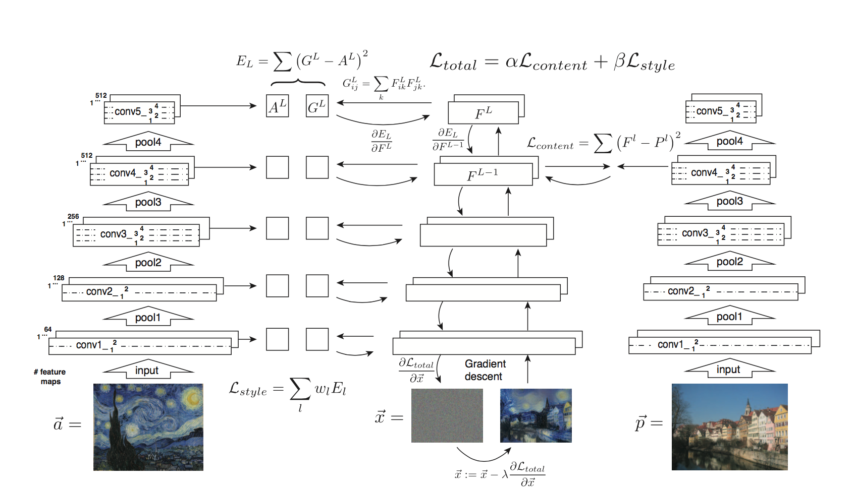
• $G^{l}_{ij}$ is the inner product between the vectorised feature maps of the initial image $i$ and $j$ in layer $l$
• $w_{l}$ is the weight of each style layers
• $A^{l}$ is that of the style image
• $F^{l}$ is layer-wise content features of the initial image
• $P^{l}$ is that of the content image

def style_content_loss(outputs):
    style_outputs = outputs['style']
    content_outputs = outputs['content']
    style_loss = tf.add_n([tf.reduce_mean((style_outputs[name]-style_targets[name])**2) 
                           for name in style_outputs.keys()])
    style_loss *= style_weight / num_style_layers

    content_loss = tf.add_n([tf.reduce_mean((content_outputs[name]-content_targets[name])**2) 
                             for name in content_outputs.keys()])
    content_loss *= content_weight / num_content_layers
    loss = style_loss + content_loss
    return loss

Run gradient descent

def clip_0_1(image):
    return tf.clip_by_value(image, clip_value_min=0.0, clip_value_max=1.0)

@tf.function()
def train_step(image):
    with tf.GradientTape() as tape:
        outputs = extractor(image)
        loss = style_content_loss(outputs)

    # tape.gradient: d_loss/d_image
    grad = tape.gradient(loss, image)
    opt.apply_gradients([(grad, image)])
    image.assign(clip_0_1(image))

style_targets = extractor(style_image)['style']
content_targets = extractor(content_image)['content']

image = tf.Variable(content_image)
opt = tf.optimizers.Adam(learning_rate=0.02, beta_1=0.99, epsilon=1e-1)
style_weight = 0    # Change it as you want
content_weight = 0  # Change it as you want

train_step(image)
train_step(image)
train_step(image)
plt.imshow(image.read_value()[0])

<matplotlib.image.AxesImage at 0x7fd5631c5d90>

Let's train with more iteration to see the results!

import time
start = time.time()

epochs = 10
steps_per_epoch = 100

step = 0
for n in range(epochs):
    for m in range(steps_per_epoch):
        step += 1
        train_step(image)
    imshow(image.read_value())
    plt.title("Train step: {}".format(step))
    plt.show()
    

end = time.time()
print("Total time: {:.1f}".format(end-start))

Total time: 27.2

Total variation loss

One downside to this basic implementation is that it produces a lot of high frequency artifacts. Decrease these using an explicit regularization term on the high frequency components of the image. In style transfer, this is often called the total variation loss:

$V(y)=\sum_i \sum_j\sqrt{(y_{i+1,j}-y_{i,j})^2 + (y_{i,j+1}-y_{i,j})^2}$

In practice, to speed up the computation, we implement the following version instead:

$V(y)=\sum_i \sum_j|y_{i+1,j}-y_{i,j}| + |y_{i,j+1}-y_{i,j}|$

This shows how the high frequency components have increased. Also, this high frequency component is basically an edge-detector. You can get similar output from the Sobel edge detector, for example:

plt.figure(figsize=(14,10))

sobel = tf.image.sobel_edges(content_image)
plt.subplot(1,2,1)
imshow(clip_0_1(sobel[...,0]/4+0.5), "Horizontal Sobel-edges")
plt.subplot(1,2,2)
imshow(clip_0_1(sobel[...,1]/4+0.5), "Vertical Sobel-edges")

def total_variation_loss(image):
    # TODO

Re-run the optimization

total_variation_weight = 0 # Change it as you want

@tf.function()
def train_step(image):
    with tf.GradientTape() as tape:
        outputs = extractor(image)
        loss = style_content_loss(outputs)
        loss += total_variation_weight*total_variation_loss(image)

    grad = tape.gradient(loss, image)
    opt.apply_gradients([(grad, image)])
    image.assign(clip_0_1(image))

image = tf.Variable(content_image)

start = time.time()

epochs = 10
steps_per_epoch = 100

step = 0
for n in range(epochs):
    for m in range(steps_per_epoch):
        step += 1
        train_step(image)
    imshow(image.read_value())
    plt.title("Train step: {}".format(step))
    plt.show()

end = time.time()
print("Total time: {:.1f}".format(end-start))

Total time: 29.2

file_name = './dataset/style_transfer_nthu_starry_night.png'
mpl.image.imsave(file_name, image[0].numpy())

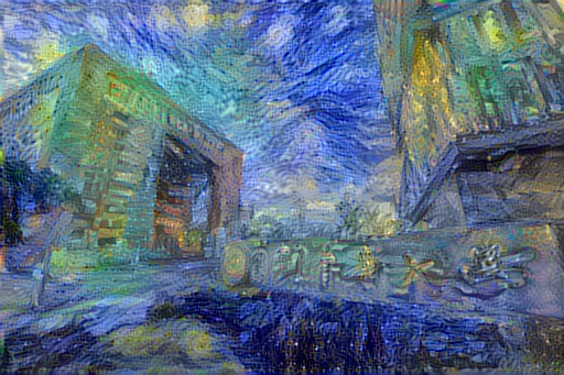
With total variational loos, the image has better quality and looks really like a masterpiece of Vincent van Gogh, right?

AdaIN

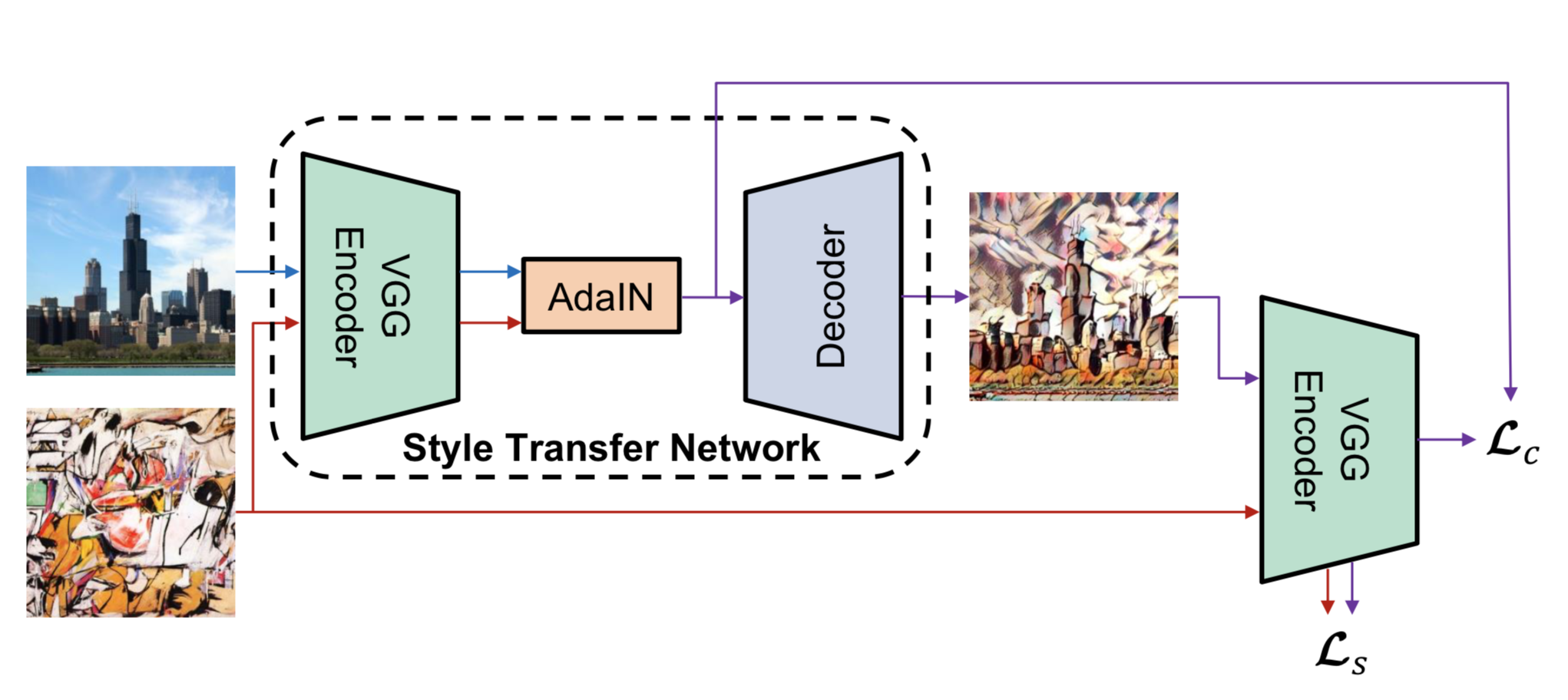
The method we mentioned above requires a slow iterative optimization process, which limits its pratical application. Xun Huang and Serge Belongie from Cornell University propose another framework, which enables arbitrary style tranfer in real-time, known as "Arbitrary Style Transfer in Real-time with Adaptive Instance Normalization".

AdaIN can transfer arbitrary new styles in real-time, combining the flexibility of the optimization-based framework and the speed similar to the fastest feed-forward approaches. At the heart of this method is a novel Adaptive Instance Normalization (AdaIN) layer aligning the mean and variance of the content features with those of the style features. Instance normalization performs style normalization by normalizing feature statistics, which have been found to carry the style information of an image in the earlier works. A decoder network is then learned to generate the final stylized image by inverting the AdaIN output back to the image space.

%matplotlib inline

CONTENT_DIRS = ['./dataset/mscoco/test2014']
STYLE_DIRS = ['./dataset/wikiart/test']

# VGG19 was trained by Caffe which converted images from RGB to BGR,
# then zero-centered each color channel with respect to the ImageNet 
# dataset, without scaling.  
IMG_MEANS = np.array([103.939, 116.779, 123.68]) # BGR

IMG_SHAPE = (224, 224, 3) # training image shape, (h, w, c)
SHUFFLE_BUFFER = 1000
BATCH_SIZE = 32
EPOCHS = 30
STEPS_PER_EPOCH = 12000 // BATCH_SIZE

Here we use MSCOCO 2014 testing dataset as our content dataset, while using WikiArt testing dataset as style dataset, containing 40,736 and 23,585 images respectively. To prevent from misunderstanding, we have to clarify the reason to use testing dataset instead of training dataset. The size of whole MSCOCO 2014 and WikiArt is more than 45G, which might be too heavy for this tutorial. In addition, our purpose is to train an style transfer model rather than image classification or object detection, thus using testing dataset is nothing to worry about.

def sample_files(dir, num, pattern='**/*.jpg'):
    '''Samples files in a directory using the reservoir sampling.'''

    paths = Path(dir).glob(pattern) # list of Path objects
    sampled = []
    for i, path in enumerate(paths):
        if i < num:
            sampled.append(path) 
        else:
            s = random.randint(0, i)
            if s < num:
                sampled[s] = path
    return sampled

def plot_images(dir, row, col, pattern):
    paths = sample_files(dir, row*col, pattern)

    plt.figure(figsize=(2*col, 2*row))
    for i in range(row*col):
        im = Image.open(paths[i])
        w, h = im.size

        plt.subplot(row, col, i+1)
        plt.imshow(im)
        plt.grid(False)
        plt.xticks([])
        plt.yticks([])
        plt.xlabel(f'{w}x{h}')
    plt.show()

print('Sampled content images:')
plot_images(CONTENT_DIRS[0], 4, 8, pattern='*.jpg')

print('Sampled style images:')
plot_images(STYLE_DIRS[0], 4, 8, pattern='*.jpg')

Sampled content images:

Sampled style images:

Dataset API

Before creating dataset API, first we have to remove some unwanted data, such as small images or grayscale images.

def clean(dir_path, min_shape=None):
    paths = Path(dir_path).glob('**/*.jpg')
    deleted  = 0
    for path in paths:
        try:
            # Make sure we can decode the image
            im = tf.io.read_file(str(path.resolve()))
            im = tf.image.decode_jpeg(im)

            # Remove grayscale images 
            shape = im.shape
            if shape[2] < 3:
                path.unlink()
                deleted += 1

            # Remove small images
            if min_shape is not None:
                if shape[0] < min_shape[0] or shape[1] < min_shape[1]:
                    path.unlink()
                    deleted += 1
        except Exception as e:
            path.unlink()
            deleted += 1
    return deleted

for dir in CONTENT_DIRS:
    deleted = clean(dir)
print(f'#Deleted content images: {deleted}')

for dir in STYLE_DIRS:
    deleted = clean(dir)
print(f'#Deleted style images: {deleted}')

#Deleted content images: 0
#Deleted style images: 0

VGG19 was trained by Caffe which converted images from RGB to BGR, then zero-centered each color channel with respect to the ImageNet dataset, without scaling. Therefore, we have to do the same thing during data preprocessing.

def preprocess_image(path, init_shape=(448, 448)):
    image = tf.io.read_file(path)
    image = tf.image.decode_jpeg(image, channels=3)
    image = tf.image.resize(image, init_shape)
    image = tf.image.random_crop(image, size=IMG_SHAPE)
    image = tf.cast(image, tf.float32)
    
    # Convert image from RGB to BGR, then zero-center each color channel with
    # respect to the ImageNet dataset, without scaling.
    image = image[..., ::-1] # RGB to BGR
    image -= (103.939, 116.779, 123.68) # BGR means
    return image

def np_image(image):
    image += (103.939, 116.779, 123.68) # BGR means
    image = image[..., ::-1] # BGR to RGB
    image = tf.clip_by_value(image, 0, 255)
    image = tf.cast(image, dtype='uint8')
    return image.numpy()

def build_dataset(num_gpus=1):
    c_paths = []
    for c_dir in CONTENT_DIRS:
        c_paths += Path(c_dir).glob('*.jpg')
    c_paths = [str(path.resolve()) for path in c_paths]
    s_paths = []
    for s_dir in STYLE_DIRS:
        s_paths += Path(s_dir).glob('*.jpg')
    s_paths = [str(path.resolve()) for path in s_paths]
    print(f'Building dataset from {len(c_paths):,} content images and {len(s_paths):,} style images... ', end='')

    AUTOTUNE = tf.data.experimental.AUTOTUNE

    c_ds = tf.data.Dataset.from_tensor_slices(c_paths)
    c_ds = c_ds.map(preprocess_image, num_parallel_calls=AUTOTUNE)
    c_ds = c_ds.repeat()
    c_ds = c_ds.shuffle(buffer_size=SHUFFLE_BUFFER)

    s_ds = tf.data.Dataset.from_tensor_slices(s_paths)
    s_ds = s_ds.map(preprocess_image, num_parallel_calls=AUTOTUNE)
    s_ds = s_ds.repeat()
    s_ds = s_ds.shuffle(buffer_size=SHUFFLE_BUFFER)

    ds = tf.data.Dataset.zip((c_ds, s_ds))
    ds = ds.batch(BATCH_SIZE * num_gpus)
    ds = ds.prefetch(buffer_size=AUTOTUNE)

    print('done')
    return ds

ds = build_dataset()
c_batch, s_batch = next(iter(ds.take(1)))

print('Content batch shape:', c_batch.shape)
print('Style batch shape:', s_batch.shape)

plt.figure(figsize=(8, 4))

plt.subplot(1, 2, 1)
plt.imshow(np_image(c_batch[0]))
plt.grid(False)
plt.xticks([])
plt.yticks([])
plt.xlabel('Content')

plt.subplot(1, 2, 2)
plt.imshow(np_image(s_batch[0]))
plt.grid(False)
plt.xticks([])
plt.yticks([])
plt.xlabel('Style')

plt.show()

Building dataset from 40,736 content images and 23,585 style images... done
Content batch shape: (32, 224, 224, 3)
Style batch shape: (32, 224, 224, 3)

Adaptive Instance Normalization

AdaIN recieves a content input $x$ and style input $y$, and simply aligns the channelwise mean and variance of $x$ to match those of $y$. It is worth knowning that unlike BN(Batch Normalization), IN(Instance Normalization) or CIN(Conditional Instance Normalization), AdaIN has no learnable affine parameters. Instead, it adaptively computes the affine parameters from the style input:

$\text{AdaIN}(x,\,y) = \sigma(y)\,(\cfrac{x - \mu(x)}{\sigma(x)}) + \mu(y)$

class AdaIN(tf.keras.layers.Layer):
    # TODO

Model

We use the first few layers of a fixed VGG-19 network to encode the content and style images. An AdaIN layer is used to perform style transfer in the feature space. A decoder is learned to invert the AdaIN output to the image spaces. Moreover, we use the same VGG encoder to compute a content loss $L_c$ and style loss $L_s$. Here we define $t$ as the output of AdaIN layer.

$t = \text{AdaIN}(f(c),\,f(s))$.

Next, we can define the loss function which is composed of content loss and style loss, where $\lambda$ is weighting factor.

$L = L_c + \lambda L_s$.

The content loss is the Euclidean distance between the target features and the features of the output image. We use the AdaIN output $t$ as the content target, instead of the commonly used feature responses of the content image. The author found this leads to slightly faster convergence and also aligns with our goal of inverting the AdaIN output $t$.

$L_c = \|\,f(g(t)) - t\,\|_2$

Since AdaIN layer only transfers the mean and standard deviation of the style features, our style loss only matches these statistics. Although we find the commonly used Gram matrix loss can produce similar results, we match the IN statistics because it is conceptually cleaner. This style loss has also been explored by Li et al.

$L_s = \sum\limits_{i=1}^{L}\|\,\mu(\phi_i(g(t)))-\mu(\phi_i(s))\,\|_2 + \sum\limits_{i=1}^{L}\|\,\sigma(\phi_i(g(t)))-\sigma(\phi_i(s))\,\|_2$

• $c$ represents content while $s$ represents style
• $t$ is the output of AdaIN layer
• $f$ is encoder
• $g$ is decoder
• $\phi_i$ denotes a layer in VGG-19 used to compute the style loss

class ArbitraryStyleTransferNet(tf.keras.Model):
    CONTENT_LAYER = 'block4_conv1'
    STYLE_LAYERS = ('block1_conv1', 'block2_conv1', 'block3_conv1', 'block4_conv1')

    @staticmethod
    def declare_decoder():
        a_input = tf.keras.Input(shape=(28, 28, 512), name='input_adain')

        h = tf.keras.layers.Conv2DTranspose(256, 3, padding='same', activation='relu')(a_input)
        h = tf.keras.layers.UpSampling2D(2)(h)
        h = tf.keras.layers.Conv2DTranspose(256, 3, padding='same', activation='relu')(h)
        h = tf.keras.layers.Conv2DTranspose(256, 3, padding='same', activation='relu')(h)
        h = tf.keras.layers.Conv2DTranspose(256, 3, padding='same', activation='relu')(h)
        h = tf.keras.layers.Conv2DTranspose(128, 3, padding='same', activation='relu')(h)
        h = tf.keras.layers.UpSampling2D(2)(h)
        h = tf.keras.layers.Conv2DTranspose(128, 3, padding='same', activation='relu')(h)
        h = tf.keras.layers.Conv2DTranspose(64, 3, padding='same', activation='relu')(h)
        h = tf.keras.layers.UpSampling2D(2)(h)
        h = tf.keras.layers.Conv2DTranspose(64, 3, padding='same', activation='relu')(h)
        output = tf.keras.layers.Conv2DTranspose(3, 3, padding='same')(h)

        return tf.keras.Model(inputs=a_input, outputs=output, name='decoder')
  
    def __init__(self,
                 img_shape=(224, 224, 3),
                 content_loss_weight=1,
                 style_loss_weight=10,
                 name='arbitrary_style_transfer_net',
                 **kwargs):
        super(ArbitraryStyleTransferNet, self).__init__(name=name, **kwargs)

        self.img_shape = img_shape
        self.content_loss_weight = content_loss_weight
        self.style_loss_weight = style_loss_weight
        
        vgg19 = tf.keras.applications.VGG19(include_top=False, weights='imagenet', input_shape=img_shape)
        vgg19.trainable = False

        c_output = [vgg19.get_layer(ArbitraryStyleTransferNet.CONTENT_LAYER).output]
        s_outputs = [vgg19.get_layer(name).output for name in ArbitraryStyleTransferNet.STYLE_LAYERS]
        self.vgg19 = tf.keras.Model(inputs=vgg19.input, outputs=c_output+s_outputs, name='vgg19')
        self.vgg19.trainable = False

        self.adain = AdaIN(name='adain')
        self.decoder = ArbitraryStyleTransferNet.declare_decoder()
  
    def call(self, inputs):
        c_batch, s_batch = inputs

        c_enc = self.vgg19(c_batch)
        c_enc_c = c_enc[0]

        s_enc = self.vgg19(s_batch)
        s_enc_c = s_enc[0]
        s_enc_s = s_enc[1:] 
        
        # normalized_c is the output of AdaIN layer
        normalized_c = self.adain((c_enc_c, s_enc_c))
        output = self.decoder(normalized_c)

        # Calculate loss
        out_enc = self.vgg19(output)
        out_enc_c = out_enc[0]
        out_enc_s = out_enc[1:]

        loss_c = tf.reduce_mean(tf.math.squared_difference(out_enc_c, normalized_c))
        self.add_loss(self.content_loss_weight * loss_c)
        
        loss_s = 0
        for o, s in zip(out_enc_s, s_enc_s):    
            o_mean, o_var = tf.nn.moments(o, axes=(1,2), keepdims=True)
            o_std = tf.sqrt(o_var + self.adain.epsilon)

            s_mean, s_var = tf.nn.moments(s, axes=(1,2), keepdims=True)
            s_std = tf.sqrt(s_var + self.adain.epsilon)

            loss_mean = tf.reduce_mean(tf.math.squared_difference(o_mean, s_mean))
            loss_std = tf.reduce_mean(tf.math.squared_difference(o_std, s_std))

            loss_s += loss_mean + loss_std
        self.add_loss(self.style_loss_weight * loss_s)

        return output, c_enc_c, normalized_c, out_enc_c

# Plot results
def plot_outputs(outputs, captions=None, col=5):
    row = len(outputs)
    plt.figure(figsize=(3*col, 3*row))
    for i in range(col):
        for j in range(row):
            plt.subplot(row, col, j*col+i+1)
            plt.imshow(np_image(outputs[j][i,...,:3]))
            plt.grid(False)
            plt.xticks([])
            plt.yticks([])
            if captions is not None:
                plt.xlabel(captions[j])
    plt.show()

ds = build_dataset()
model = ArbitraryStyleTransferNet(img_shape=IMG_SHAPE)

c_batch, s_batch = next(iter(ds.take(1)))
print(f'Input shape: ({c_batch.shape}, {s_batch.shape})')
output, *_ = model((c_batch, s_batch))
print(f'Output shape: {output.shape}')
print(f'Init. content loss: {model.losses[0]:,.2f}, style loss: {model.losses[1]:,.2f}')
model.summary()

Building dataset from 40,736 content images and 23,585 style images... done
Input shape: ((32, 224, 224, 3), (32, 224, 224, 3))
Output shape: (32, 224, 224, 3)
Init. content loss: 2,172,319.75, style loss: 15,373,436.00
Model: "arbitrary_style_transfer_net"
_________________________________________________________________
Layer (type)                 Output Shape              Param #   
=================================================================
vgg19 (Model)                [(None, 28, 28, 512), (No 3505728   
_________________________________________________________________
adain (AdaIN)                multiple                  0         
_________________________________________________________________
decoder (Model)              (None, 224, 224, 3)       3505219   
=================================================================
Total params: 7,010,947
Trainable params: 3,505,219
Non-trainable params: 3,505,728
_________________________________________________________________

Training

# Train the model
optimizer = tf.keras.optimizers.Adam(learning_rate=5e-4)
c_loss_metric, s_loss_metric = tf.keras.metrics.Mean(), tf.keras.metrics.Mean()

CKP_DIR = 'checkpoints'
init_epoch = 1

ckp = tf.train.latest_checkpoint(CKP_DIR)
if ckp:
    model.load_weights(ckp)
    init_epoch = int(ckp.split('_')[-1]) + 1
    print(f'Resume training from epoch {init_epoch-1}')

ERROR:tensorflow:Couldn't match files for checkpoint checkpoints/ckpt_4

@tf.function
def train_step(inputs):
    with tf.GradientTape() as tape:
        model(inputs)
        c_loss, s_loss = model.losses
        loss = c_loss + s_loss
    grads = tape.gradient(loss, model.trainable_variables)
    optimizer.apply_gradients(zip(grads, model.trainable_variables))

    c_loss_metric(c_loss)
    s_loss_metric(s_loss)

def train(dataset, init_epoch):
    for epoch in range(init_epoch, EPOCHS+1):
        print(f'Epoch {epoch:>2}/{EPOCHS}')
        for step, inputs in enumerate(ds.take(STEPS_PER_EPOCH)):
            train_step(inputs)
            print(f'{step+1:>5}/{STEPS_PER_EPOCH} - loss: {c_loss_metric.result()+s_loss_metric.result():,.2f} - content loss: {c_loss_metric.result():,.2f} - style loss: {s_loss_metric.result():,.2f}', end='\r') 

        print()
        model.save_weights(os.path.join(CKP_DIR, f'ckpt_{epoch}'))
        c_loss_metric.reset_states()
        s_loss_metric.reset_states()

        output, c_enc_c, normalized_c, out_enc_c = model((c_batch, s_batch))
        plot_outputs((s_batch, c_batch, output, c_enc_c, normalized_c, out_enc_c), 
                     ('Style', 'Content', 'Trans', 'Content Enc', 'Normalized', 'Trans Enc'))

train(ds, init_epoch)

Epoch  1/30
  500/500 - loss: 2,086,217.88 - content loss: 624,608.75 - style loss: 1,461,609.120000

Epoch  2/30
  500/500 - loss: 1,037,496.31 - content loss: 438,236.50 - style loss: 599,259.81

Epoch  3/30
  351/500 - loss: 892,105.88 - content loss: 394,261.66 - style loss: 497,844.19

Testing

CKP_DIR = 'checkpoints/ckpt_20'

model = ArbitraryStyleTransferNet(img_shape=IMG_SHAPE)
model.load_weights(CKP_DIR)

ds = build_dataset()

for idx, (c_batch, s_batch) in enumerate(ds):
    if idx > 1:
        break
    output, c_enc_c, normalized_c, out_enc_c = model((c_batch, s_batch))
    print('Recovered loss:', tf.reduce_sum(model.losses).numpy())

    plot_outputs((s_batch, c_batch, output), ('Style', 'Content', 'Trans'))

Building dataset from 40,736 content images and 23,585 style images... done
Recovered loss: 445823.38

Recovered loss: 341863.44

NTHU Example

One of the most important advantages of AdaIN is speed. Earlier we have implemented iterative style transfer, which takes roughly 30 seconds per image on Nvidia GeForce RTX 2080Ti, meanwhile AdaIN is up to three orders of magnitude faster than the former. Here we demostrate the power of AdaIN with single content and 25 distinct styles.

def preprocess_example(path, init_shape=(IMG_SHAPE[0], IMG_SHAPE[1])):
    image = tf.io.read_file(path)
    image = tf.image.decode_jpeg(image, channels=3)
    image = tf.image.resize(image, init_shape)
    image = tf.cast(image, tf.float32)
    
    # Convert image from RGB to BGR, then zero-center each color channel with
    # respect to the ImageNet dataset, without scaling.
    image = image[..., ::-1] # RGB to BGR
    image -= (103.939, 116.779, 123.68) # BGR means
    return image

def nthu_example(num_gpus=1):
    c_paths = ['./dataset/content_nthu.jpg']
    
    s_paths = []
    for s_dir in STYLE_DIRS:
        s_paths += Path(s_dir).glob('*.jpg')
    s_paths = [str(path.resolve()) for path in s_paths]
    print(f'Building dataset from {len(c_paths):,} content images and {len(s_paths):,} style images... ', end='')
    
    AUTOTUNE = tf.data.experimental.AUTOTUNE
    
    c_ds = tf.data.Dataset.from_tensor_slices(c_paths)
    c_ds = c_ds.map(preprocess_example, num_parallel_calls=AUTOTUNE)
    c_ds = c_ds.repeat()
    c_ds = c_ds.shuffle(buffer_size=SHUFFLE_BUFFER)
    
    s_ds = tf.data.Dataset.from_tensor_slices(s_paths)
    s_ds = s_ds.map(preprocess_image, num_parallel_calls=AUTOTUNE)
    s_ds = s_ds.repeat()
    s_ds = s_ds.shuffle(buffer_size=SHUFFLE_BUFFER)
    
    ds = tf.data.Dataset.zip((c_ds, s_ds))
    ds = ds.batch(BATCH_SIZE * num_gpus)
    ds = ds.prefetch(buffer_size=AUTOTUNE)
    
    print('done')
    return ds

ds = nthu_example()
outputs = []

for idx, (c_batch, s_batch) in enumerate(ds):
    if idx > 4:
        break
    output, c_enc_c, normalized_c, out_enc_c = model((c_batch, s_batch))
    outputs.append(output)
    
plot_outputs((outputs))

Building dataset from 1 content images and 23,585 style images... done

Save and Load Models

Model progress can be saved during and after training. This means a model can resume where it left off and avoid long training times. Saving also means you can share your model and others can recreate your work. When publishing research models and techniques, most machine learning practitioners share:

• code to create the model, and
• the trained weights, or parameters, for the model

Sharing this data helps others understand how the model works and try it themselves with new data.

The phrase "Saving a Tensorflow model" typically means one of two things:

1. Checkpoints, OR
2. SavedModel.

Checkpoints capture the exact value of all parameters (tf.Variable objects) used by a model. Checkpoints do not contain any description of the computation defined by the model and thus are typically only useful when source code that will use the saved parameter values is available.

The SavedModel format on the other hand includes a serialized description of the computation defined by the model in addition to the parameter values (checkpoint). Models in this format are independent of the source code that created the model. They are thus suitable for deployment via TensorFlow Serving, TensorFlow Lite, TensorFlow.js, or programs in other programming languages (the C, C++, Java, Go, Rust, C# etc. TensorFlow APIs). Saving a fully-functional model is very useful - you can load them in TensorFlow.js and then train and run them in web browsers, or convert them to run on mobile devices using TensorFlow Lite.

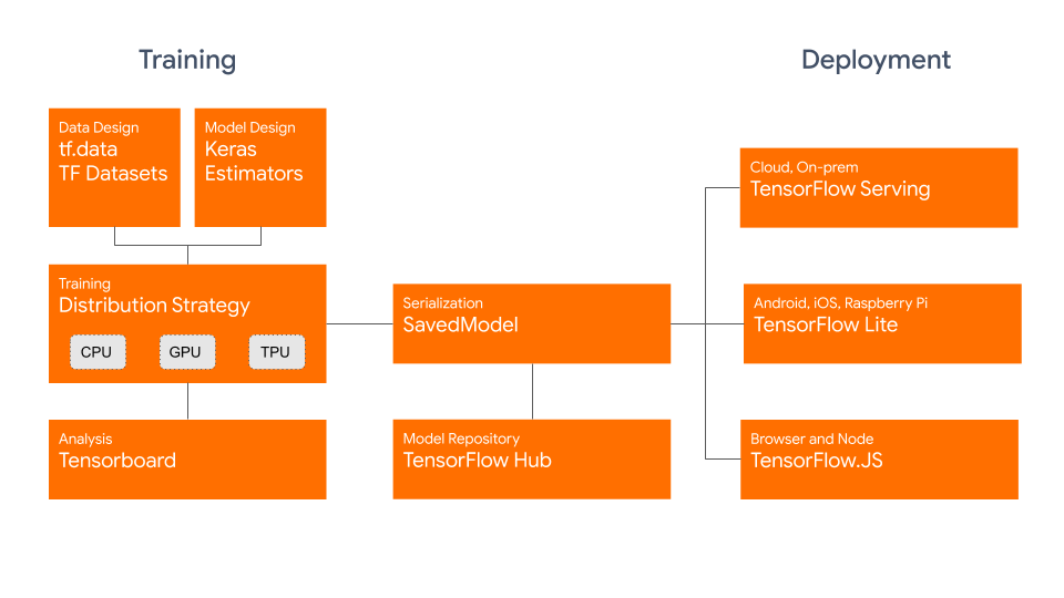
Example of the graph defined by the model, which is visualized by TensorBoard.

Inside checkpoints

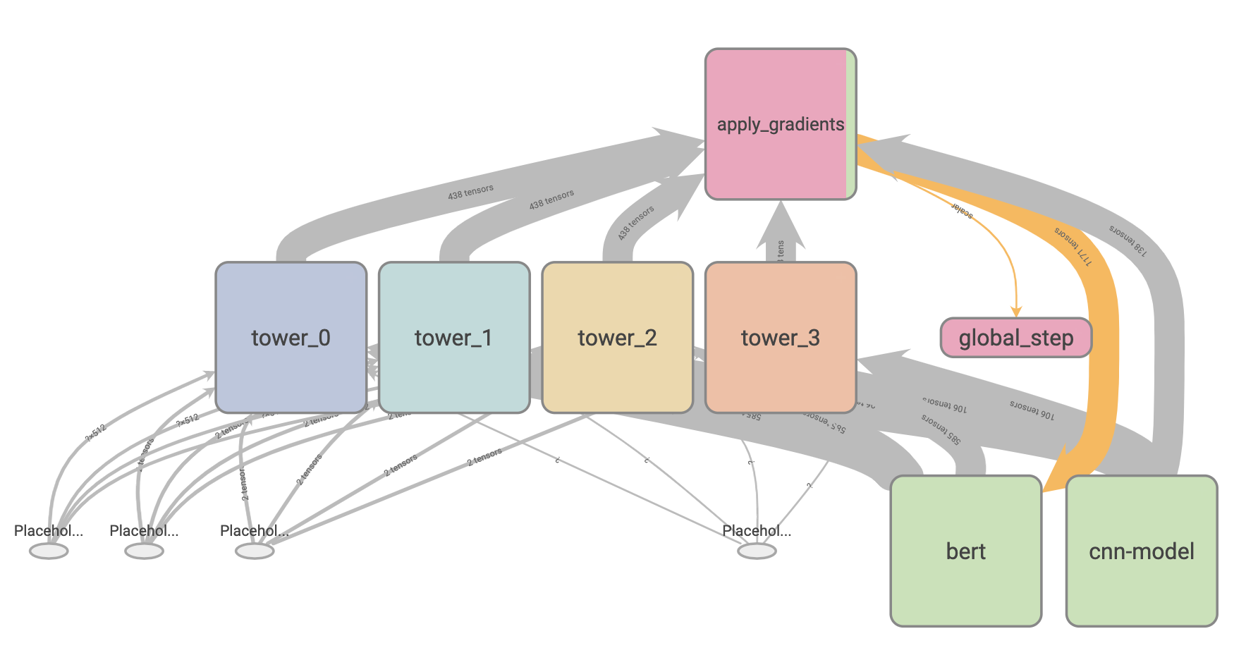
Before starting this tutorial, you should know what kinds of information are stored in the checkpoints. There are various parameters used by the model, including hyperparameters, weights and optimizer slot variables. TensorFlow matches variables to checkpointed values by traversing a directed graph with named edges, starting from the object being loaded. Edge names typically come from attribute names in objects.

The dependency graph looks like this:

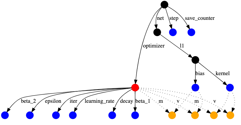
With the optimizer in red, regular variables in blue, and optimizer slot variables in orange. The other nodes, for example representing the tf.train.Checkpoint, are black.

Slot variables are part of the optimizer's state, but are created for a specific variable. For example the 'm' edges above correspond to momentum, which the Adam optimizer tracks for each variable. Slot variables are only saved in a checkpoint if the variable and the optimizer would both be saved, thus the dashed edges.

This tutorial covers APIs for writing and reading checkpoints. For more information about SavedModel API, see Using the SavedModel format and Save and load models guides.

There are several ways to save TensorFlow models, depending on the API you are using. In this section, we are going to demonstrate

• tf.keras.callbacks.ModelCheckpoint
• Model.save_weights
• tf.train.Checkpoints

For simplicity, here we use MNIST dataset to demonstrate how to save and load wegihts.

import os

(train_images, train_labels), (test_images, test_labels) = tf.keras.datasets.mnist.load_data()

train_labels = train_labels[:1000]
test_labels = test_labels[:1000]

train_images = train_images[:1000].reshape(-1, 28 * 28) / 255.0
test_images = test_images[:1000].reshape(-1, 28 * 28) / 255.0

class MyModel(tf.keras.Model):
    def __init__(self):
        super(MyModel, self).__init__()
        self.flatten = tf.keras.layers.Flatten()
        self.dropout = tf.keras.layers.Dropout(0.2)
        self.d1 = tf.keras.layers.Dense(128, activation='relu')
        self.d2 = tf.keras.layers.Dense(10, activation='softmax')

    def call(self, x):
        x = self.flatten(x)
        x = self.d1(x)
        x = self.dropout(x)
        return self.d2(x)

tf.keras.backend.clear_session()
model = MyModel()
model.build(input_shape=(None, 28, 28))
model.summary()

WARNING:tensorflow:Unresolved object in checkpoint: (root)._callable_losses
WARNING:tensorflow:Unresolved object in checkpoint: (root)._eager_losses
WARNING:tensorflow:A checkpoint was restored (e.g. tf.train.Checkpoint.restore or tf.keras.Model.load_weights) but not all checkpointed values were used. See above for specific issues. Use expect_partial() on the load status object, e.g. tf.train.Checkpoint.restore(...).expect_partial(), to silence these warnings, or use assert_consumed() to make the check explicit. See https://www.tensorflow.org/alpha/guide/checkpoints#loading_mechanics for details.
Model: "my_model"
_________________________________________________________________
Layer (type)                 Output Shape              Param #   
=================================================================
flatten (Flatten)            multiple                  0         
_________________________________________________________________
dropout (Dropout)            multiple                  0         
_________________________________________________________________
dense (Dense)                multiple                  100480    
_________________________________________________________________
dense_1 (Dense)              multiple                  1290      
=================================================================
Total params: 101,770
Trainable params: 101,770
Non-trainable params: 0
_________________________________________________________________

Save checkpoints during training

You can use a trained model without having to retrain it, or pick-up training where you left off - in case the training process was interrupted. The tf.keras.callbacks.ModelCheckpoint callback allows to continually save the model both during and at the end of training, and this method saves all parameters used by a model, including weights and optimizer. The callback provides several options to create unique names for checkpoints and adjust the checkpointing frequency.

Checkpoint callback usage

EPOCHS = 5

# Checkpoint path and its name
CKP_DIR_SAVE_CALLBACKS = './checkpoints_save_callbacks/ckpt-{epoch}.ckpt'
checkpoint_dir = os.path.dirname(CKP_DIR_SAVE_CALLBACKS)

model.compile(optimizer='adam',
              loss='sparse_categorical_crossentropy',
              metrics=['accuracy'])

# Create a callback that saves the model's weights every 1 epochs
cp_callback = tf.keras.callbacks.ModelCheckpoint(
    filepath=CKP_DIR_SAVE_CALLBACKS, 
    verbose=1, 
    save_weights_only=True,
    period=1)

# Train the model with the new callback
model.fit(train_images, 
          train_labels,
          epochs=EPOCHS, 
          callbacks=[cp_callback],
          validation_data=(test_images,test_labels))

WARNING:tensorflow:`period` argument is deprecated. Please use `save_freq` to specify the frequency in number of samples seen.
Train on 1000 samples, validate on 1000 samples
Epoch 1/5
 672/1000 [===================>..........] - ETA: 0s - loss: 1.7914 - accuracy: 0.4301 
Epoch 00001: saving model to ./checkpoints_save_callbacks/ckpt-1.ckpt
1000/1000 [==============================] - 1s 876us/sample - loss: 1.5585 - accuracy: 0.5360 - val_loss: 1.0544 - val_accuracy: 0.7210
Epoch 2/5
 672/1000 [===================>..........] - ETA: 0s - loss: 0.7181 - accuracy: 0.8229
Epoch 00002: saving model to ./checkpoints_save_callbacks/ckpt-2.ckpt
1000/1000 [==============================] - 0s 169us/sample - loss: 0.6965 - accuracy: 0.8200 - val_loss: 0.7100 - val_accuracy: 0.7920
Epoch 3/5
 640/1000 [==================>...........] - ETA: 0s - loss: 0.4567 - accuracy: 0.8797
Epoch 00003: saving model to ./checkpoints_save_callbacks/ckpt-3.ckpt
1000/1000 [==============================] - 0s 168us/sample - loss: 0.4774 - accuracy: 0.8650 - val_loss: 0.5816 - val_accuracy: 0.8260
Epoch 4/5
 704/1000 [====================>.........] - ETA: 0s - loss: 0.3987 - accuracy: 0.8807
Epoch 00004: saving model to ./checkpoints_save_callbacks/ckpt-4.ckpt
1000/1000 [==============================] - 0s 177us/sample - loss: 0.3816 - accuracy: 0.8940 - val_loss: 0.5167 - val_accuracy: 0.8420
Epoch 5/5
 704/1000 [====================>.........] - ETA: 0s - loss: 0.3153 - accuracy: 0.9219
Epoch 00005: saving model to ./checkpoints_save_callbacks/ckpt-5.ckpt
1000/1000 [==============================] - 0s 166us/sample - loss: 0.3180 - accuracy: 0.9200 - val_loss: 0.4693 - val_accuracy: 0.8550

<tensorflow.python.keras.callbacks.History at 0x7fd480115810>

Now rebuild a fresh, untrained model, and evaluate it on the test set. An untrained model will perform at chance levels (~10% accuracy):

# Create a new model instance
model = MyModel()
model.compile(optimizer='adam',
              loss='sparse_categorical_crossentropy',
              metrics=['accuracy'])

# Re-evaluate the model
loss, acc = model.evaluate(test_images,  test_labels, verbose=2)
print("Restored model, accuracy: {:5.2f}%".format(100*acc))

1000/1 - 0s - loss: 2.5291 - accuracy: 0.1040
Restored model, accuracy: 10.40%

Create a new, untrained model. When restoring a model from weights-only, you must have a model with the same architecture as the original model. Since it's the same model architecture, you can share weights despite that it's a different instance of the model.

After loading the weights from the checkpoint, we can re-evaluate the model. As you can see, the accuracy raises up to 85.5%, which is same as the one we have trained earlier.

# Load the previously saved weights
latest = tf.train.latest_checkpoint(checkpoint_dir)
model.load_weights(latest)

# Re-evaluate the model
loss, acc = model.evaluate(test_images,  test_labels, verbose=2)
print("Restored model, accuracy: {:5.2f}%".format(100*acc))

1000/1 - 0s - loss: 0.5423 - accuracy: 0.8550
Restored model, accuracy: 85.50%

What are these files?

The above code stores the weights to a collection of checkpoint-formatted files that contain only the trained weights in a binary format. Checkpoints contain: * One or more shards that contain your model's weights. * An index file that indicates which weights are stored in a which shard.

Manually save weights

We just demonstrated how to save and load the weights into a model when using Model.fit. Manually saving them is just as simple with the Model.save_weights method, and it is quite useful during custom training. In our Deep Learning course, most of assignments and competitions are required custom training.

mnist = tf.keras.datasets.mnist

(x_train, y_train), (x_test, y_test) = mnist.load_data()
x_train, x_test = x_train / 255.0, x_test / 255.0

train_ds = tf.data.Dataset.from_tensor_slices((x_train, y_train)).shuffle(10000).batch(32)
test_ds = tf.data.Dataset.from_tensor_slices((x_test, y_test)).batch(32)

tf.keras.backend.clear_session()
model = MyModel()

loss_object = tf.keras.losses.SparseCategoricalCrossentropy()
optimizer = tf.keras.optimizers.Adam()

train_loss = tf.keras.metrics.Mean(name='train_loss')
train_accuracy = tf.keras.metrics.SparseCategoricalAccuracy(name='train_accuracy')
test_loss = tf.keras.metrics.Mean(name='test_loss')
test_accuracy = tf.keras.metrics.SparseCategoricalAccuracy(name='test_accuracy')

@tf.function
def train_step(images, labels):
    with tf.GradientTape() as tape:
        predictions = model(images)
        loss = loss_object(labels, predictions)
    gradients = tape.gradient(loss, model.trainable_variables)
    optimizer.apply_gradients(zip(gradients, model.trainable_variables))

    train_loss(loss)
    train_accuracy(labels, predictions)
    
@tf.function
def test_step(images, labels):
    predictions = model(images)
    t_loss = loss_object(labels, predictions)

    test_loss(t_loss)
    test_accuracy(labels, predictions)

Another thing you should notice is the difference between tf.keras.callbacks.ModelCheckpoint and Model.save_weights. The former one saves all parameters used in model, inclusing weights and optimizers, while the latter one only saves weights. No information about optimizer is saved. Therefore, if you restore the checkpoints saved by Model.save_weights method, it is not possible to pick-up training where you left off exactly. Fortunately, in most cases, information relevant to optimizer is not that important comparing to weights. In addition, since Model.save_weights only stores weights, the checkpoint files are lighter than the one created by tf.kears.callbacks.ModelCheckpoint.

CKP_DIR_SAVE_WEIGHTS = './checkpoints_save_weights'

for epoch in range(EPOCHS):
    for images, labels in train_ds:
        train_step(images, labels)

    for test_images, test_labels in test_ds:
        test_step(test_images, test_labels)

    template = 'Epoch {:0}, Loss: {:.2f}, Accuracy: {:.2f}, Test Loss: {:.2f}, Test Accuracy: {:.2f}'
    print (template.format(epoch+1,
                           train_loss.result(),
                           train_accuracy.result()*100,
                           test_loss.result(),
                           test_accuracy.result()*100))
    
    # Use Model.save_weights during training
    # You can modify the saving frequency by simply using "if epoch == ?, then save"
    print("Saved checkpoint for step {}: {}".format(int(epoch+1), CKP_DIR_SAVE_WEIGHTS + f'/ckpt-{epoch+1}'))
    model.save_weights(os.path.join(CKP_DIR_SAVE_WEIGHTS, f'ckpt-{epoch}'))

    # Reset the metrics for the next epoch
    train_loss.reset_states()
    train_accuracy.reset_states()
    test_loss.reset_states()
    test_accuracy.reset_states()

WARNING:tensorflow:Layer my_model is casting an input tensor from dtype float64 to the layer's dtype of float32, which is new behavior in TensorFlow 2.  The layer has dtype float32 because it's dtype defaults to floatx.

If you intended to run this layer in float32, you can safely ignore this warning. If in doubt, this warning is likely only an issue if you are porting a TensorFlow 1.X model to TensorFlow 2.

To change all layers to have dtype float64 by default, call `tf.keras.backend.set_floatx('float64')`. To change just this layer, pass dtype='float64' to the layer constructor. If you are the author of this layer, you can disable autocasting by passing autocast=False to the base Layer constructor.

Epoch 1, Loss: 0.26, Accuracy: 92.73, Test Loss: 0.13, Test Accuracy: 96.05
Saved checkpoint for step 1: ./checkpoints_save_weights/ckpt-1
Epoch 2, Loss: 0.11, Accuracy: 96.67, Test Loss: 0.10, Test Accuracy: 96.94
Saved checkpoint for step 2: ./checkpoints_save_weights/ckpt-2
Epoch 3, Loss: 0.08, Accuracy: 97.66, Test Loss: 0.09, Test Accuracy: 97.16
Saved checkpoint for step 3: ./checkpoints_save_weights/ckpt-3
Epoch 4, Loss: 0.06, Accuracy: 98.22, Test Loss: 0.09, Test Accuracy: 97.46
Saved checkpoint for step 4: ./checkpoints_save_weights/ckpt-4
Epoch 5, Loss: 0.05, Accuracy: 98.59, Test Loss: 0.08, Test Accuracy: 97.53
Saved checkpoint for step 5: ./checkpoints_save_weights/ckpt-5

# Create a new model instance
model = MyModel()

Here you might encounter FailedPreconditionError. Please recompile the cell containing def train_step and def test_step, and then run the following cells.

for test_images, test_labels in test_ds:
    test_step(test_images, test_labels)

template = 'Test Loss: {:.2f}, Test Accuracy: {:.2f}'
print (template.format(test_loss.result(), test_accuracy.result()*100))

test_loss.reset_states()
test_accuracy.reset_states()

WARNING:tensorflow:Layer my_model_1 is casting an input tensor from dtype float64 to the layer's dtype of float32, which is new behavior in TensorFlow 2.  The layer has dtype float32 because it's dtype defaults to floatx.

If you intended to run this layer in float32, you can safely ignore this warning. If in doubt, this warning is likely only an issue if you are porting a TensorFlow 1.X model to TensorFlow 2.

To change all layers to have dtype float64 by default, call `tf.keras.backend.set_floatx('float64')`. To change just this layer, pass dtype='float64' to the layer constructor. If you are the author of this layer, you can disable autocasting by passing autocast=False to the base Layer constructor.

Test Loss: 2.39, Test Accuracy: 14.19

# Restore the weights
model.load_weights('checkpoints_save_weights/ckpt-4')

for test_images, test_labels in test_ds:
    test_step(test_images, test_labels)

template = 'Test Loss: {:.2f}, Test Accuracy: {:.2f}'
print (template.format(test_loss.result(), test_accuracy.result()*100))

test_loss.reset_states()
test_accuracy.reset_states()

Test Loss: 0.08, Test Accuracy: 97.53

Manually checkpointing

Another way to save checkpoint during custom training is to use tf.train.Checkpoint API, capturing the exact value of all parameters used by model. It is distinct from Model.save_weights, which saves only weights but the optimizer.

# Create a new model instance
tf.keras.backend.clear_session()
model = MyModel()

To manually make a checkpoint you will need a tf.train.Checkpoint object. Where the objects you want to checkpoint are set as attributes on the object.

A tf.train.CheckpointManager can also be helpful for managing multiple checkpoints.

CKP_DIR_SAVE_CHECKPOINTS = './checkpoints_save_checkpoints'

# Place the models and optimizers you want to store 
# as the arguments of tf.train.Checkpoint
# You can store several different models and optimizers at the same time
ckpt = tf.train.Checkpoint(step=tf.Variable(1), optimizer=optimizer, model=model)
manager = tf.train.CheckpointManager(ckpt, CKP_DIR_SAVE_CHECKPOINTS, max_to_keep=3)

for epoch in range(EPOCHS):
    for images, labels in train_ds:
        train_step(images, labels)

    for test_images, test_labels in test_ds:
        test_step(test_images, test_labels)
        
    template = 'Epoch {:0}, Loss: {:.2f}, Accuracy: {:.2f}, Test Loss: {:.2f}, Test Accuracy: {:.2f}'
    print (template.format(epoch+1,
                           train_loss.result(),
                           train_accuracy.result()*100,
                           test_loss.result(),
                           test_accuracy.result()*100))
    
    # save checkpoint for each epoch
    if int(ckpt.step) % 1 == 0:
        save_path = manager.save()
        print("Saved checkpoint for step {}: {}".format(int(ckpt.step), save_path))
    
    ckpt.step.assign_add(1)

    # Reset the metrics for the next epoch
    train_loss.reset_states()
    train_accuracy.reset_states()
    test_loss.reset_states()
    test_accuracy.reset_states()

WARNING:tensorflow:Layer my_model is casting an input tensor from dtype float64 to the layer's dtype of float32, which is new behavior in TensorFlow 2.  The layer has dtype float32 because it's dtype defaults to floatx.

If you intended to run this layer in float32, you can safely ignore this warning. If in doubt, this warning is likely only an issue if you are porting a TensorFlow 1.X model to TensorFlow 2.

To change all layers to have dtype float64 by default, call `tf.keras.backend.set_floatx('float64')`. To change just this layer, pass dtype='float64' to the layer constructor. If you are the author of this layer, you can disable autocasting by passing autocast=False to the base Layer constructor.

Epoch 1, Loss: 0.19, Accuracy: 94.29, Test Loss: 0.12, Test Accuracy: 96.58
Saved checkpoint for step 1: ./checkpoints_save_checkpoints/ckpt-1
Epoch 2, Loss: 0.09, Accuracy: 97.26, Test Loss: 0.09, Test Accuracy: 97.22
Saved checkpoint for step 2: ./checkpoints_save_checkpoints/ckpt-2
Epoch 3, Loss: 0.06, Accuracy: 98.08, Test Loss: 0.09, Test Accuracy: 97.27
Saved checkpoint for step 3: ./checkpoints_save_checkpoints/ckpt-3
Epoch 4, Loss: 0.05, Accuracy: 98.48, Test Loss: 0.08, Test Accuracy: 97.60
Saved checkpoint for step 4: ./checkpoints_save_checkpoints/ckpt-4
Epoch 5, Loss: 0.04, Accuracy: 98.83, Test Loss: 0.07, Test Accuracy: 97.79
Saved checkpoint for step 5: ./checkpoints_save_checkpoints/ckpt-5

model = MyModel()

for test_images, test_labels in test_ds:
    test_step(test_images, test_labels)

template = 'Test Loss: {:.2f}, Test Accuracy: {:.2f}'
print (template.format(test_loss.result(), test_accuracy.result()*100))

test_loss.reset_states()
test_accuracy.reset_states()

WARNING:tensorflow:Layer my_model_1 is casting an input tensor from dtype float64 to the layer's dtype of float32, which is new behavior in TensorFlow 2.  The layer has dtype float32 because it's dtype defaults to floatx.

If you intended to run this layer in float32, you can safely ignore this warning. If in doubt, this warning is likely only an issue if you are porting a TensorFlow 1.X model to TensorFlow 2.

To change all layers to have dtype float64 by default, call `tf.keras.backend.set_floatx('float64')`. To change just this layer, pass dtype='float64' to the layer constructor. If you are the author of this layer, you can disable autocasting by passing autocast=False to the base Layer constructor.

WARNING:tensorflow:Unresolved object in checkpoint: (root).optimizer.iter
WARNING:tensorflow:Unresolved object in checkpoint: (root).optimizer.beta_1
WARNING:tensorflow:Unresolved object in checkpoint: (root).optimizer.beta_2
WARNING:tensorflow:Unresolved object in checkpoint: (root).optimizer.decay
WARNING:tensorflow:Unresolved object in checkpoint: (root).optimizer.learning_rate
WARNING:tensorflow:A checkpoint was restored (e.g. tf.train.Checkpoint.restore or tf.keras.Model.load_weights) but not all checkpointed values were used. See above for specific issues. Use expect_partial() on the load status object, e.g. tf.train.Checkpoint.restore(...).expect_partial(), to silence these warnings, or use assert_consumed() to make the check explicit. See https://www.tensorflow.org/alpha/guide/checkpoints#loading_mechanics for details.
Test Loss: 2.33, Test Accuracy: 13.89

After the first you can pass a new model and manager, but pickup training exactly where you left off.

# To load checkpoints back to our new model, you have to create another 
# "tf.train.Checkpoint" for new model and optimizer
ckpt = tf.train.Checkpoint(step=tf.Variable(1), optimizer=optimizer, model=model)
manager = tf.train.CheckpointManager(ckpt, CKP_DIR_SAVE_CHECKPOINTS, max_to_keep=3)
ckpt.restore(manager.latest_checkpoint)

for test_images, test_labels in test_ds:
    test_step(test_images, test_labels)

template = 'Test Loss: {:.2f}, Test Accuracy: {:.2f}'
print (template.format(test_loss.result(), test_accuracy.result()*100))

test_loss.reset_states()
test_accuracy.reset_states()

Test Loss: 0.07, Test Accuracy: 97.79

For more information about tf.train.Checkpoint and the detailed structure of saved checkpoints, please check Training checkpoints guide.

Reference

• VGG 19 model.

• The code of style transfer is based on Tersorflow official tutorial, while the code of visualization is based on How to Visualize Filters and Feature Maps in Convolutional Neural Networks by Jason Brownlee.

• The original paper of style transfer implemented in this tutorial is A Neural Algorithm of Artistic Style by Gatys et al.

• The orifinal paper of AdaIN implemented in this tutorial is "Arbitrary Style Transfer in Real-time with Adaptive Instance Normalization" by Huang et al.

• Original work of Style Transfer's TensorFlow implementation is from Anish Athalye's GitHub account anishathalye.

• The tutorial of "Save and Load Model" is based on Tensorflow official tutorial.

Assignment

In this assignment, you need to do following things:

Part I (A Neural Algorithm of Artistic Style)

1. Implement total variational loss. tf.image.total_variation is not allowed (10%).
2. Change the weights for the style, content, and total variational loss (10%).
3. Use other layers in the model (10%).
   • You need to calculate both content loss and style loss from different layers in the model
4. Write a brief report. Explain how the results are affected when you change the weights, use different layers for calculating loss (10%).
   • Insert markdown cells in the notebook to write the report.

Part II (AdaIN)

1. Implement AdaIN layer and use single content image to create 25 images with different styles (60%).

You can dowaload WikiArt and MSCOCO 2014 from here.

Requirements:

• Submit your code file Lab11-2_{student id}.ipynb and result images.
• Honest code. Students will get 0 if plagiarism is found.
• Deadline: 2024-11-07 (Thur) 00:00.