Sequence to sequence learning (Seq2Seq) is about training models to convert sequences from one domain (e.g. sentences in Chinese) to sequences in another domain (e.g. the same sentences translated to English). This can be used for machine translation, free-form question answering (generating a natural language answer given a natural language question), text summarization, and image captioning. In general, it is applicable any time you need to generate text.
In this lab, we will introduce how to train a seq2seq model for Chinese to English translation. After training the model in this notebook, you will be able to input a Chinese sentence, such as "你今晚會去派對嗎?", and return the English translation: "will you go to the party tonight?".
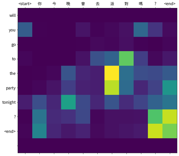
The translation quality is reasonable for a toy example, but the generated attention plot is perhaps more interesting. This shows which parts of the input sentence has the model's attention while translating:
Seq2Seq Learning
Encoder-Decoder Architecture
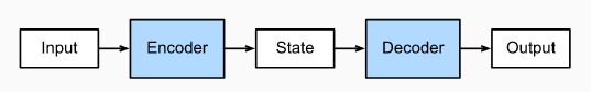
The encoder-decoder architecture is a neural network design pattern. In this architecture, the network is partitioned into two parts, the encoder and the decoder. The encoder’s role is encoding the inputs into hidden state, or hidden representation, which often contains several tensors. Then the hidden state is passed into the decoder to generate the outputs.
Sequence to Sequence
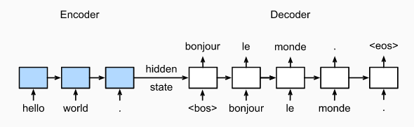
The sequence to sequence (seq2seq) model is based on the encoder-decoder architecture to generate a sequence output for a sequence input, where both the encoder and the decoder tend to both be recurrent neural networks (RNNs). The hidden state of the encoder is used directly to initialize the hidden state of decoder, bringing information from the encoder to the decoder. In machine translation, the encoder transforms a source sentence, i.e. “你今晚會去派對嗎?”, into hidden state, which is a vector, that captures its semantic information. The decoder then uses this state to generate the translated target sentence, e.g. “will you go to the party tonight?”.
Sequence to Sequence with Attention Mechanism
Now, let’s talk about the attention mechanism. What is it and why do we need it?
Let’s use Neural Machine Translation (NMT) as an example. In NMT, the encoder maps the meaning of a sentence into a fixed-length hidden representation, this representation is expected to be a good summary of the entire input sequence, where the decoder can generate a corresponding translation based on that vector.
A critical and apparent disadvantage of this fixed-length context vector design is the incapability of the system to remember longer sequences. It is common to see that the fixed-length vector forgot the earlier parts of the input sentence once it has processed the entire input. A solution we proposed in Bahdanau et al., 2014 and Luong et al., 2015.. These papers introduced and refined a technique called Attention, which highly improved the quality of machine translation systems. Attention allows the model to focus on the relevant parts of the input sequence as needed.
That was the idea behind Attention! It can be illustrated as follows:
Details of attention
Notations:
- $T_x$: the length of the input
- $h_j$: the $j_{th}$ hidden state of the encdoer
- $s_i$: the $i_{th}$ hidden state of the decoder
- $c_i$: context vector, a sum of hidden states of the input sequence, weighted by alignment scores
- $a$: alighment(match) score function, calculate the match score between two vectors($s_{i-1}$ and $h_j$)
- $e_{ij}$: alighment(match) score between the $s_{i-1}$ and $h_j$
- $\alpha_{ij}$: softmax of the alignment(match) score
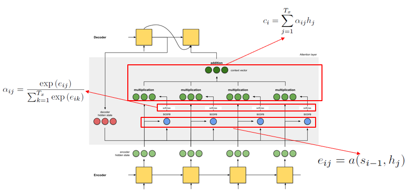
And there are many types of score function:
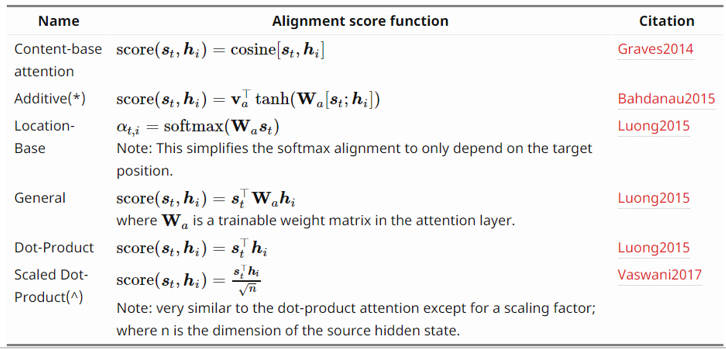
For more details, please read this blog: Attn: Illustrated Attention
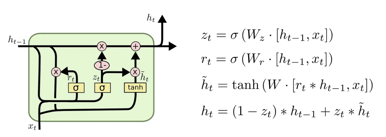
Gated Recurrent Unit (GRU)
Teacher Forcing
Teacher forcing is an efficient and effective method used widely in the training process of recurrent neural networks, which uses the ground truth from a previous time step as the input to the next time step.
Neural Machine Translation
Next, we will show how to train a seq2seq model using a translation dataset (Chinese to English), and then we will demonstrate some results of the translation to evaluate the model. In this lab, we will use GRU layers.
import os
os.environ['TF_CPP_MIN_LOG_LEVEL'] = '3'
import warnings
warnings.filterwarnings("ignore")

import tensorflow as tf
import matplotlib.pyplot as plt
import matplotlib.ticker as ticker
import unicodedata
import re
import numpy as np
import os
import time
from sklearn.model_selection import train_test_split

from pylab import *
from matplotlib.font_manager import FontProperties
gpus = tf.config.experimental.list_physical_devices('GPU')
if gpus:
    try:
        # Restrict TensorFlow to only use the first GPU
        tf.config.experimental.set_visible_devices(gpus[0], 'GPU')

        # Currently, memory growth needs to be the same across GPUs
        for gpu in gpus:
            tf.config.experimental.set_memory_growth(gpu, True)
        logical_gpus = tf.config.experimental.list_logical_devices('GPU')
        print(len(gpus), "Physical GPUs,", len(logical_gpus), "Logical GPUs")
    except RuntimeError as e:
        # Memory growth must be set before GPUs have been initialized
        print(e)
1 Physical GPUs, 1 Logical GPUs
Prepare the dataset
# dataset path
# use the Chinese-English dataset
path_to_file = "./data/eng-chinese.txt"
Data preprocessing
- Add a start and end token to each sentence.
- Clean the sentences by removing special characters.
- Create a word index and reverse word index (dictionaries mapping from word → id and id → word).
- Pad each sentence to a maximum length.
def unicode_to_ascii(s):
    return ''.join(c for c in unicodedata.normalize('NFD', s)
                   if unicodedata.category(c) != 'Mn')


def preprocess_eng(w):
    w = unicode_to_ascii(w.lower().strip())

    # creating a space between a word and the punctuation following it
    # eg: "he is a boy." => "he is a boy ."
    # Reference:- https://stackoverflow.com/questions/3645931/
    # python-padding-punctuation-with-white-spaces-keeping-punctuation
    w = re.sub(r"([?.!,])", r" \1 ", w)
    # replace several spaces with one space
    w = re.sub(r'[" "]+', " ", w)

    # replacing everything with space except (a-z, A-Z, ".", "?", "!", ",")
    w = re.sub(r"[^a-zA-Z?.!,]+", " ", w)
    w = w.rstrip().strip()

    # adding a start and an end token to the sentence
    # so that the model know when to start and stop predicting.
    w = '<start> ' + w + ' <end>'
    return w


def preprocess_chinese(w):
    w = unicode_to_ascii(w.lower().strip())
    w = re.sub(r'[" "]+', "", w)
    w = w.rstrip().strip()
    w = " ".join(list(w))  # add the space between words
    w = '<start> ' + w + ' <end>'
    return w
# u means unicode encoder
en_sentence = u"May I borrow this book?"
chn_sentence = u"我可以借這本書麼?"
print(preprocess_eng(en_sentence))
print(preprocess_chinese(chn_sentence))
print(preprocess_chinese(chn_sentence).encode('utf-8'))
<start> may i borrow this book ? <end>
<start> 我 可 以 借 這 本 書 麼 ? <end>
b'<start> \xe6\x88\x91 \xe5\x8f\xaf \xe4\xbb\xa5 \xe5\x80\x9f \xe9\x80\x99 \xe6\x9c\xac \xe6\x9b\xb8 \xe9\xba\xbc \xef\xbc\x9f <end>'
# 1. Remove the accents
# 2. Clean the sentences
# 3. Return word pairs in the format: [ENGLISH, CHINESE]
def create_dataset(path, num_examples=None):
    lines = open(path, encoding='UTF-8').read().strip().split('\n')
    word_pairs = [[w for w in l.split('\t')] for l in lines[:num_examples]]
    word_pairs = [[preprocess_eng(w[0]), preprocess_chinese(w[1])]
                  for w in word_pairs]

    # return two tuple: one tuple includes all English sentenses, and
    # another tuple includes all Chinese sentenses
    return word_pairs


word_pairs = create_dataset(path_to_file)
# show the first twenty examples
word_pairs[:20]
[['<start> hi . <end>', '<start> 嗨 。 <end>'],
 ['<start> hi . <end>', '<start> 你 好 。 <end>'],
 ['<start> run . <end>', '<start> 你 用 跑 的 。 <end>'],
 ['<start> wait ! <end>', '<start> 等 等 ! <end>'],
 ['<start> hello ! <end>', '<start> 你 好 。 <end>'],
 ['<start> i try . <end>', '<start> 让 我 来 。 <end>'],
 ['<start> i won ! <end>', '<start> 我 赢 了 。 <end>'],
 ['<start> oh no ! <end>', '<start> 不 会 吧 。 <end>'],
 ['<start> cheers ! <end>', '<start> 乾 杯 ! <end>'],
 ['<start> he ran . <end>', '<start> 他 跑 了 。 <end>'],
 ['<start> hop in . <end>', '<start> 跳 进 来 。 <end>'],
 ['<start> i lost . <end>', '<start> 我 迷 失 了 。 <end>'],
 ['<start> i quit . <end>', '<start> 我 退 出 。 <end>'],
 ['<start> i m ok . <end>', '<start> 我 沒 事 。 <end>'],
 ['<start> listen . <end>', '<start> 听 着 。 <end>'],
 ['<start> no way ! <end>', '<start> 不 可 能 ! <end>'],
 ['<start> no way ! <end>', '<start> 没 门 ! <end>'],
 ['<start> really ? <end>', '<start> 你 确 定 ? <end>'],
 ['<start> try it . <end>', '<start> 试 试 吧 。 <end>'],
 ['<start> we try . <end>', '<start> 我 们 来 试 试 。 <end>']]
en, chn = zip(*create_dataset(path_to_file))
print(en[-1])
print(chn[-1])
# show the size of the dataset
assert len(en) == len(chn)
print("Size:", len(en))
<start> if a person has not had a chance to acquire his target language by the time he s an adult , he s unlikely to be able to reach native speaker level in that language . <end>
<start> 如 果 一 個 人 在 成 人 前 沒 有 機 會 習 得 目 標 語 言 , 他 對 該 語 言 的 認 識 達 到 母 語 者 程 度 的 機 會 是 相 當 小 的 。 <end>
Size: 20289
def max_length(tensor):
    # padding the sentence to max_length
    return max(len(t) for t in tensor)

def tokenize(lang):
    lang_tokenizer = tf.keras.preprocessing.text.Tokenizer(
        filters='')
    # generate a dictionary, e.g. word -> index(of the dictionary)
    lang_tokenizer.fit_on_texts(lang)

    # output the vector sequences, e.g. [1, 7, 237, 3, 2]
    tensor = lang_tokenizer.texts_to_sequences(lang)

    # padding sentences to the same length
    tensor = tf.keras.preprocessing.sequence.pad_sequences(tensor,
                                                           padding='post')
    return tensor, lang_tokenizer

def load_dataset(path, num_examples=None):
    # creating cleaned input, output pairs
    # regard Chinese as source sentence, regard English as target sentence
    targ_lang, inp_lang = zip(*create_dataset(path, num_examples))

    input_tensor, inp_lang_tokenizer = tokenize(inp_lang)
    target_tensor, targ_lang_tokenizer = tokenize(targ_lang)

    return input_tensor, target_tensor, inp_lang_tokenizer, targ_lang_tokenizer
# Try experimenting with the size of that dataset
# num_examples = 10000, if num examples = None means no limitation
num_examples = None
input_tensor, target_tensor, inp_lang, targ_lang = load_dataset(
    path_to_file, num_examples)

# Calculate max_length of the target tensors
max_length_targ, max_length_inp = max_length(
    target_tensor), max_length(input_tensor)

# Creating training and validation sets using an 95-5 split
input_tensor_train, input_tensor_val, target_tensor_train, target_tensor_val = train_test_split(
    input_tensor, target_tensor, test_size=0.05)

# Show length of the training data and validation data
print("# training data: {:d}\n# test data: {:d}".format(len(input_tensor_train), len(input_tensor_val)))
# training data: 19274
# test data: 1015
def convert(lang, tensor):
    for t in tensor:
        if t != 0:
            print("%d ----> %s" % (t, lang.index_word[t]))

print("Input Language; index to word mapping")
convert(inp_lang, input_tensor_train[0])
print()
print("Target Language; index to word mapping")
convert(targ_lang, target_tensor_train[0])
Input Language; index to word mapping
1 ----> <start>
9 ----> 不
19 ----> 要
224 ----> 放
1235 ----> 棄
108 ----> 英
125 ----> 語
3 ----> 。
2 ----> <end>

Target Language; index to word mapping
1 ----> <start>
31 ----> don
12 ----> t
611 ----> quit
79 ----> english
3 ----> .
2 ----> <end>
Create a tf.data dataset
BUFFER_SIZE = len(input_tensor_train)
BATCH_SIZE = 128
steps_per_epoch = len(input_tensor_train)//BATCH_SIZE
embedding_dim = 256
units = 1024
# 0 is a reserved index that won't be assigned to any word, so the size of vocabulary should add 1
vocab_inp_size = len(inp_lang.word_index) + 1
vocab_tar_size = len(targ_lang.word_index) + 1

dataset = tf.data.Dataset.from_tensor_slices(
    (input_tensor_train, target_tensor_train)).shuffle(BUFFER_SIZE)
dataset = dataset.batch(BATCH_SIZE, drop_remainder=True)

example_input_batch, example_target_batch = next(iter(dataset))
example_input_batch.shape, example_target_batch.shape
(TensorShape([128, 46]), TensorShape([128, 38]))
Encoder
class Encoder(tf.keras.Model):
    def __init__(self, vocab_size, embedding_dim, enc_units, batch_sz):
        # vacab_size=vocab_inp_size=9394, embedding_dim=256 enc_units=1024 batch_sz=128
        super(Encoder, self).__init__()
        self.batch_sz = batch_sz
        self.enc_units = enc_units
        self.embedding = tf.keras.layers.Embedding(vocab_size, embedding_dim)
        self.gru = tf.keras.layers.GRU(self.enc_units,
                                       return_sequences=True,
                                       return_state=True,
                                       recurrent_activation='sigmoid',
                                       recurrent_initializer='glorot_uniform')

    def call(self, x, hidden):
        # x is the training data with shape == (batch_size, max_length)  -> (128, 46)
        # which means there are batch_size sentences in one batch, the length of each sentence is max_length
        # hidden state shape == (batch_size, units) -> (128, 1024)
        # after embedding, x shape == (batch_size, max_length, embedding_dim) -> (128, 46, 256)
        x = self.embedding(x)

        # output contains the state(in GRU, the hidden state and the output are same) from all timestamps,
        # output shape == (batch_size, max_length, units) -> (128, 46, 1024)
        # state is the hidden state of the last timestamp, shape == (batch_size, units) -> (128, 1024)
        output, state = self.gru(x, initial_state=hidden)

        return output, state

    def initialize_hidden_state(self):
        # initialize the first state of the gru,  shape == (batch_size, units) -> (128, 1024)
        return tf.zeros((self.batch_sz, self.enc_units))
encoder = Encoder(vocab_inp_size, embedding_dim, units, BATCH_SIZE)

# sample input
sample_hidden = encoder.initialize_hidden_state()
sample_output, sample_hidden = encoder(example_input_batch, sample_hidden)
print('Encoder output shape: (batch size, sequence length, units) {}'.format(sample_output.shape))
print('Encoder Hidden state shape: (batch size, units) {}'.format(sample_hidden.shape))

# the output and the hidden state of GRU is equal
print(sample_output[-1, -1, :] == sample_hidden[-1, :])
Encoder output shape: (batch size, sequence length, units) (128, 46, 1024)
Encoder Hidden state shape: (batch size, units) (128, 1024)
tf.Tensor([ True  True  True ...  True  True  True], shape=(1024,), dtype=bool)
Attention
In this lab, we use the Bahdanau Attention as our attention mechanism. The formula of score function in Bahdanau Attention is:
$$\text{score}(s_t, h_i) = v_a^T\tanh (W_a[s_t; h_i])$$class BahdanauAttention(tf.keras.Model):
def __init__(self, units):
super(BahdanauAttention, self).__init__()
self.W1 = tf.keras.layers.Dense(units)
self.W2 = tf.keras.layers.Dense(units)
self.V = tf.keras.layers.Dense(1)
def call(self, query, values):
# query shape == (batch_size, hidden size)
# hidden_with_time_axis shape == (batch_size, 1, hidden size)
# we are doing this to perform addition to calculate the score
hidden_with_time_axis = tf.expand_dims(query, 1)
# score shape == (batch_size, max_length, 1)
# we get 1 at the last axis because we are applying score to self.V
# the shape of the tensor before applying self.V is (batch_size, max_length, units)
score = self.V(tf.nn.tanh(self.W1(values) + self.W2(hidden_with_time_axis)))
# attention_weights shape == (batch_size, max_length, 1)
attention_weights = tf.nn.softmax(score, axis=1)
# context_vector shape == (batch_size, max_length, hidden_size)
context_vector = attention_weights * values
# context_vector shape after sum == (batch_size, hidden_size)
context_vector = tf.reduce_sum(context_vector, axis=1)
return context_vector, attention_weights
attention_layer = BahdanauAttention(10)
attention_result, attention_weights = attention_layer(sample_hidden, sample_output)

print("Attention result shape: (batch size, units) {}".format(attention_result.shape))
print("Attention weights shape: (batch_size, sequence_length, 1) {}".format(attention_weights.shape))
Attention result shape: (batch size, units) (128, 1024)
Attention weights shape: (batch_size, sequence_length, 1) (128, 46, 1)
Decoder
class Decoder(tf.keras.Model):
    def __init__(self, vocab_size, embedding_dim, dec_units, batch_sz):
        # vocab_size=vocab_tar_size=6082, embedding_dim=256, dec_units=1024, batch_sz=128
        super(Decoder, self).__init__()
        self.batch_sz = batch_sz
        self.dec_units = dec_units
        self.embedding = tf.keras.layers.Embedding(vocab_size, embedding_dim)
        self.gru = tf.keras.layers.GRU(self.dec_units,
                                       return_sequences=True,
                                       return_state=True,
                                       recurrent_initializer='glorot_uniform')
        # the dimension of the output is the vocab size, through the softmax function,
        # this layer will return the probability of each word in the dictory
        self.fc = tf.keras.layers.Dense(vocab_size)

        # used for attention
        self.attention = BahdanauAttention(self.dec_units)

    def call(self, x, hidden, enc_output):
        # This function outputs a result at each timestamp
        # The hidden state of fisrt timestamp in the decoder is
        # the hidden state of last timestamp in the encoder
        context_vector, attention_weights = self.attention(hidden, enc_output)

        # x shape after passing through embedding == (batch_size, 1, embedding_dim)
        x = self.embedding(x)

        # concatenate the input x and the context_vector, as the input of the GRU
        # context_vector shape == (batch_size, units) -> (128, 1024)
        # x shape after concatenation == (batch_size, 1, embedding_dim + hidden_size) -> (128, 1, 1024 + 256)
        x = tf.concat([tf.expand_dims(context_vector, 1), x], axis=-1)

        # passing the concatenated vector to the GRU
        # get the output and state of the current timestamp
        # output shape == (batch_size, 1, units) -> (128, 1, 1024)
        # state shape == (batch_size, units) -> (128, 1024)
        output, state = self.gru(x)

        # output shape == (batch_size, hidden_size) -> (128, 1024)
        output = tf.reshape(output, (-1, output.shape[2]))

        # output shape == (batch_size, vocab) -> (128, 6082)
        x = self.fc(output)

        return x, state, attention_weights
decoder = Decoder(vocab_tar_size, embedding_dim, units, BATCH_SIZE)
sample_decoder_output, _, _ = decoder(tf.random.uniform((BATCH_SIZE, 1)), sample_hidden, sample_output)
print('Decoder output shape: (batch_size, vocab size) {}'.format(sample_decoder_output.shape))
Decoder output shape: (batch_size, vocab size) (128, 6082)
Define the optimizer and the loss function
optimizer = tf.keras.optimizers.Adam()
loss_object = tf.keras.losses.SparseCategoricalCrossentropy(from_logits=True, reduction='none')

def loss_function(real, pred):
    """Calculate the loss value
    Args:
        real: the true label  shape == (batch_size,) -> (128,)
        pred: the probability of each word from the vocabulary, is the output from the decoder
                 shape == (batch_size, vocab_size) -> (128, 6082)

    Returns:
        the average loss of the data in a batch size
    """
    mask = tf.math.logical_not(tf.math.equal(real, 0))
    loss_ = loss_object(real, pred)

    mask = tf.cast(mask, dtype=loss_.dtype)
    loss_ *= mask

    return tf.reduce_mean(loss_)
Checkpoints (Object-based saving)
checkpoint_dir = './checkpoints/chinese-eng'
checkpoint_prefix = os.path.join(checkpoint_dir, "ckpt")
checkpoint = tf.train.Checkpoint(optimizer=optimizer,
                                 encoder=encoder,
                                 decoder=decoder)
Training
- Pass the input through the encoder which return encoder output and the encoder hidden state.
- The encoder output, encoder hidden state and the decoder input (which is the start token) is passed to the decoder.
- The decoder returns the predictions and the decoder hidden state.
- The decoder hidden state is then passed back into the model and the predictions are used to calculate the loss.
- Use teacher forcing to decide the next input to the decoder.
- Teacher forcing is the technique where the target word is passed as the next input to the decoder.
- The final step is to calculate the gradients and apply it to the optimizer and backpropagate.
@tf.function
def train_step(inp, targ, enc_hidden):
    loss = 0

    with tf.GradientTape() as tape:
        enc_output, enc_hidden = encoder(inp, enc_hidden)

        dec_hidden = enc_hidden

        # feed the <start> as the first input of the decoder
        # dec input shape == (batch_size, 1) -> (128, 1)
        dec_input = tf.expand_dims([targ_lang.word_index['<start>']] * BATCH_SIZE, 1)

        # Teacher forcing - feeding the target as the next input
        # because of the data preprocessing(add a start token to the sentence)
        # the first word is <start>, so t starts from 1(not 0)
        for t in range(1, targ.shape[1]):
            # passing enc_output to the decoder
            predictions, dec_hidden, _ = decoder(dec_input, dec_hidden, enc_output)

            # targ[:, t] is the true label(index of the word) of every sentence(in a batch)
            # at the current timestamp
            # like [  85   18   25   25  ···  1047   79   13], shape == (batch_size,) -> (128,)
            # predictions shape == (batch_size, vocab_size) -> (128, 6082)
            loss += loss_function(targ[:, t], predictions)

            # using teacher forcing
            dec_input = tf.expand_dims(targ[:, t], 1)

    batch_loss = (loss / int(targ.shape[1]))

    # collect all trainable variables
    variables = encoder.trainable_variables + decoder.trainable_variables

    # calculate the gradients for the whole variables
    gradients = tape.gradient(loss, variables)

    # apply the gradients on the variables
    optimizer.apply_gradients(zip(gradients, variables))

    return batch_loss
You don't need to train the model by yourself, you can download the model weights here.
# set the epochs for training
EPOCHS = 50

for epoch in range(EPOCHS):
    start = time.time()

    # get the initial hidden state of gru
    enc_hidden = encoder.initialize_hidden_state()
    total_loss = 0

    for (batch, (inp, targ)) in enumerate(dataset.take(steps_per_epoch)):
        batch_loss = train_step(inp, targ, enc_hidden)
        total_loss += batch_loss

        if batch % 100 == 0:
            print('Epoch {} Batch {} Loss {:.4f}'.format(epoch + 1,
                                                         batch,
                                                         batch_loss.numpy()))

    # saving (checkpoint) the model every 5 epochs
    if (epoch + 1) % 5 == 0:
        checkpoint.save(file_prefix=checkpoint_prefix)

    print('Epoch {} Loss {:.4f}'.format(epoch + 1, total_loss / steps_per_epoch))
    print('Time taken for 1 epoch {} sec\n'.format(time.time() - start))
Epoch 1 Batch 0 Loss 2.0672
Epoch 1 Batch 100 Loss 1.0858
Epoch 1 Loss 1.1569
Time taken for 1 epoch 67.52481317520142 sec

Epoch 2 Batch 0 Loss 0.9404
Epoch 2 Batch 100 Loss 0.8437
Epoch 2 Loss 0.9176
Time taken for 1 epoch 42.66153526306152 sec

Epoch 3 Batch 0 Loss 0.8847
Epoch 3 Batch 100 Loss 0.7639
Epoch 3 Loss 0.7906
Time taken for 1 epoch 42.7527289390564 sec

Epoch 4 Batch 0 Loss 0.7008
Epoch 4 Batch 100 Loss 0.7006
Epoch 4 Loss 0.7083
Time taken for 1 epoch 42.78386306762695 sec

Epoch 5 Batch 0 Loss 0.6397
Epoch 5 Batch 100 Loss 0.6498
Epoch 5 Loss 0.6394
Time taken for 1 epoch 42.983898878097534 sec

Epoch 6 Batch 0 Loss 0.5845
Epoch 6 Batch 100 Loss 0.5558
Epoch 6 Loss 0.5717
Time taken for 1 epoch 42.796711683273315 sec

Epoch 7 Batch 0 Loss 0.5106
Epoch 7 Batch 100 Loss 0.4862
Epoch 7 Loss 0.5051
Time taken for 1 epoch 42.725685358047485 sec

Epoch 8 Batch 0 Loss 0.4111
Epoch 8 Batch 100 Loss 0.4354
Epoch 8 Loss 0.4400
Time taken for 1 epoch 42.741515159606934 sec

Epoch 9 Batch 0 Loss 0.3577
Epoch 9 Batch 100 Loss 0.3517
Epoch 9 Loss 0.3778
Time taken for 1 epoch 42.724628925323486 sec

Epoch 10 Batch 0 Loss 0.3143
Epoch 10 Batch 100 Loss 0.3086
Epoch 10 Loss 0.3202
Time taken for 1 epoch 42.88447189331055 sec

Epoch 11 Batch 0 Loss 0.2356
Epoch 11 Batch 100 Loss 0.2685
Epoch 11 Loss 0.2696
Time taken for 1 epoch 42.666970014572144 sec

Epoch 12 Batch 0 Loss 0.2124
Epoch 12 Batch 100 Loss 0.2199
Epoch 12 Loss 0.2247
Time taken for 1 epoch 42.62536382675171 sec

Epoch 13 Batch 0 Loss 0.1735
Epoch 13 Batch 100 Loss 0.1899
Epoch 13 Loss 0.1825
Time taken for 1 epoch 43.02557921409607 sec

Epoch 14 Batch 0 Loss 0.1483
Epoch 14 Batch 100 Loss 0.1648
Epoch 14 Loss 0.1476
Time taken for 1 epoch 42.63216209411621 sec

Epoch 15 Batch 0 Loss 0.1086
Epoch 15 Batch 100 Loss 0.1140
Epoch 15 Loss 0.1169
Time taken for 1 epoch 42.81301736831665 sec

Epoch 16 Batch 0 Loss 0.0833
Epoch 16 Batch 100 Loss 0.0970
Epoch 16 Loss 0.0906
Time taken for 1 epoch 42.649391412734985 sec

Epoch 17 Batch 0 Loss 0.0597
Epoch 17 Batch 100 Loss 0.0597
Epoch 17 Loss 0.0696
Time taken for 1 epoch 42.95430898666382 sec

Epoch 18 Batch 0 Loss 0.0434
Epoch 18 Batch 100 Loss 0.0405
Epoch 18 Loss 0.0525
Time taken for 1 epoch 42.668476819992065 sec

Epoch 19 Batch 0 Loss 0.0458
Epoch 19 Batch 100 Loss 0.0441
Epoch 19 Loss 0.0394
Time taken for 1 epoch 42.678829193115234 sec

Epoch 20 Batch 0 Loss 0.0267
Epoch 20 Batch 100 Loss 0.0318
Epoch 20 Loss 0.0307
Time taken for 1 epoch 43.19267010688782 sec

Epoch 21 Batch 0 Loss 0.0217
Epoch 21 Batch 100 Loss 0.0285
Epoch 21 Loss 0.0247
Time taken for 1 epoch 42.72158074378967 sec

Epoch 22 Batch 0 Loss 0.0191
Epoch 22 Batch 100 Loss 0.0194
Epoch 22 Loss 0.0196
Time taken for 1 epoch 42.796473264694214 sec

Epoch 23 Batch 0 Loss 0.0144
Epoch 23 Batch 100 Loss 0.0175
Epoch 23 Loss 0.0158
Time taken for 1 epoch 42.88829517364502 sec

Epoch 24 Batch 0 Loss 0.0106
Epoch 24 Batch 100 Loss 0.0119
Epoch 24 Loss 0.0139
Time taken for 1 epoch 42.81622910499573 sec

Epoch 25 Batch 0 Loss 0.0136
Epoch 25 Batch 100 Loss 0.0168
Epoch 25 Loss 0.0130
Time taken for 1 epoch 43.19053649902344 sec

Epoch 26 Batch 0 Loss 0.0090
Epoch 26 Batch 100 Loss 0.0104
Epoch 26 Loss 0.0122
Time taken for 1 epoch 42.69778561592102 sec

Epoch 27 Batch 0 Loss 0.0114
Epoch 27 Batch 100 Loss 0.0111
Epoch 27 Loss 0.0122
Time taken for 1 epoch 42.79571199417114 sec

Epoch 28 Batch 0 Loss 0.0135
Epoch 28 Batch 100 Loss 0.0130
Epoch 28 Loss 0.0150
Time taken for 1 epoch 42.76797008514404 sec

Epoch 29 Batch 0 Loss 0.0144
Epoch 29 Batch 100 Loss 0.0237
Epoch 29 Loss 0.0193
Time taken for 1 epoch 42.71591567993164 sec

Epoch 30 Batch 0 Loss 0.0124
Epoch 30 Batch 100 Loss 0.0149
Epoch 30 Loss 0.0171
Time taken for 1 epoch 42.99852180480957 sec

Epoch 31 Batch 0 Loss 0.0147
Epoch 31 Batch 100 Loss 0.0211
Epoch 31 Loss 0.0161
Time taken for 1 epoch 42.9156436920166 sec

Epoch 32 Batch 0 Loss 0.0144
Epoch 32 Batch 100 Loss 0.0088
Epoch 32 Loss 0.0133
Time taken for 1 epoch 42.92474126815796 sec

Epoch 33 Batch 0 Loss 0.0063
Epoch 33 Batch 100 Loss 0.0077
Epoch 33 Loss 0.0111
Time taken for 1 epoch 42.80640244483948 sec

Epoch 34 Batch 0 Loss 0.0111
Epoch 34 Batch 100 Loss 0.0088
Epoch 34 Loss 0.0103
Time taken for 1 epoch 42.72117829322815 sec

Epoch 35 Batch 0 Loss 0.0116
Epoch 35 Batch 100 Loss 0.0150
Epoch 35 Loss 0.0099
Time taken for 1 epoch 42.8981568813324 sec

Epoch 36 Batch 0 Loss 0.0097
Epoch 36 Batch 100 Loss 0.0066
Epoch 36 Loss 0.0092
Time taken for 1 epoch 43.09346604347229 sec

Epoch 37 Batch 0 Loss 0.0085
Epoch 37 Batch 100 Loss 0.0098
Epoch 37 Loss 0.0092
Time taken for 1 epoch 42.70402550697327 sec

Epoch 38 Batch 0 Loss 0.0056
Epoch 38 Batch 100 Loss 0.0093
Epoch 38 Loss 0.0094
Time taken for 1 epoch 42.623132944107056 sec

Epoch 39 Batch 0 Loss 0.0054
Epoch 39 Batch 100 Loss 0.0064
Epoch 39 Loss 0.0092
Time taken for 1 epoch 42.727014780044556 sec

Epoch 40 Batch 0 Loss 0.0071
Epoch 40 Batch 100 Loss 0.0086
Epoch 40 Loss 0.0093
Time taken for 1 epoch 42.96038866043091 sec

Epoch 41 Batch 0 Loss 0.0086
Epoch 41 Batch 100 Loss 0.0079
Epoch 41 Loss 0.0098
Time taken for 1 epoch 42.88073968887329 sec

Epoch 42 Batch 0 Loss 0.0048
Epoch 42 Batch 100 Loss 0.0085
Epoch 42 Loss 0.0110
Time taken for 1 epoch 42.68013620376587 sec

Epoch 43 Batch 0 Loss 0.0073
Epoch 43 Batch 100 Loss 0.0083
Epoch 43 Loss 0.0108
Time taken for 1 epoch 42.810646295547485 sec

Epoch 44 Batch 0 Loss 0.0077
Epoch 44 Batch 100 Loss 0.0094
Epoch 44 Loss 0.0107
Time taken for 1 epoch 42.75139260292053 sec

Epoch 45 Batch 0 Loss 0.0043
Epoch 45 Batch 100 Loss 0.0128
Epoch 45 Loss 0.0113
Time taken for 1 epoch 42.889697790145874 sec

Epoch 46 Batch 0 Loss 0.0077
Epoch 46 Batch 100 Loss 0.0176
Epoch 46 Loss 0.0112
Time taken for 1 epoch 42.79266571998596 sec

Epoch 47 Batch 0 Loss 0.0086
Epoch 47 Batch 100 Loss 0.0068
Epoch 47 Loss 0.0109
Time taken for 1 epoch 42.78707766532898 sec

Epoch 48 Batch 0 Loss 0.0081
Epoch 48 Batch 100 Loss 0.0139
Epoch 48 Loss 0.0099
Time taken for 1 epoch 42.75366759300232 sec

Epoch 49 Batch 0 Loss 0.0065
Epoch 49 Batch 100 Loss 0.0061
Epoch 49 Loss 0.0099
Time taken for 1 epoch 42.72990894317627 sec

Epoch 50 Batch 0 Loss 0.0093
Epoch 50 Batch 100 Loss 0.0091
Epoch 50 Loss 0.0093
Time taken for 1 epoch 42.9361207485199 sec
Translate
- The evaluate function is similar to the training loop, except we don't use teacher forcing here. The input to the decoder at each time step is its previous predictions along with the hidden state and the encoder output.
- Stop predicting when the model predicts the end token.
- And store the attention weights for every time step.
Note:
- In the
plot_attention function, you need to change thefont = FontProperties(fname=r"./data/TaipeiSansTCBeta-Regular.ttf", size=14), where fname denotes the location of the font, based on your computer. Otherwise, the Chinese character will not be displayed in the plot.
def evaluate(sentence):
    """Translate a sentence
    Args:
        sentence: the test sentence
    """

    # max_length_targ 38, max_length_inp 64
    attention_plot = np.zeros((max_length_targ, max_length_inp))

    sentence = preprocess_chinese(sentence)

    # convert each word to the index in the test sentence
    inputs = [inp_lang.word_index[i] for i in sentence.split(' ')]
    inputs = tf.keras.preprocessing.sequence.pad_sequences([inputs],
                                                           maxlen=max_length_inp,
                                                           padding='post')

    inputs = tf.convert_to_tensor(inputs)

    result = ''

    # hidden shape == (1, 1024)
    hidden = [tf.zeros((1, units))]

    # enc out shape == (1, max_length_inp, 1024) -> (1, 46, 1024)
    # enc hidden shape == (1, 1024)
    enc_out, enc_hidden = encoder(inputs, hidden)

    dec_hidden = enc_hidden
    dec_input = tf.expand_dims([targ_lang.word_index['<start>']], 0)

    for t in range(max_length_targ):
        predictions, dec_hidden, attention_weights = decoder(dec_input, dec_hidden, enc_out)

        # storing the attention weigths to plot later on
        attention_weights = tf.reshape(attention_weights, (-1, ))
        attention_plot[t] = attention_weights.numpy()

        # get the index which has the highest probability
        predicted_id = tf.argmax(predictions[0]).numpy()
        #  convert the index to the word
        result += targ_lang.index_word[predicted_id] + ' '

        # when the decoder predicts the end, stop prediction
        if targ_lang.index_word[predicted_id] == '<end>':
            return result, sentence, attention_plot

        # the predicted id is fed back into the model
        dec_input = tf.expand_dims([predicted_id], 0)

    return result, sentence, attention_plot


# function for plotting the attention weights
def plot_attention(attention, sentence, predicted_sentence):
    # you need to change the fname based on your system, and the Chinese can be displayed in the plot
    font = FontProperties(fname=r"./data/TaipeiSansTCBeta-Regular.ttf", size=14)
    fig = plt.figure(figsize=(10, 10))
    ax = fig.add_subplot(1, 1, 1)
    ax.matshow(attention, cmap='viridis')

    fontdict = {'fontsize': 14}

    # set the x-tick/y-tick labels with list of string labels
    ax.set_xticklabels([''] + sentence, fontdict=fontdict, fontproperties=font)
    ax.set_yticklabels([''] + predicted_sentence, fontdict=fontdict, fontproperties=font)

    # set tick locators
    ax.xaxis.set_major_locator(ticker.MultipleLocator(1))
    ax.yaxis.set_major_locator(ticker.MultipleLocator(1))
    plt.show()

def translate(sentence):
    result, sentence, attention_plot = evaluate(sentence)
    print('Input: %s' % (sentence))
    print('Predicted translation: {}'.format(result))

    attention_plot = attention_plot[:len(result.split(' ')), :len(sentence.split(' '))]
    plot_attention(attention_plot, sentence.split(' '), result.split(' '))
Restore the latest checkpoint and test
checkpoint_dir = './checkpoints/chinese-eng'
print(tf.train.latest_checkpoint(checkpoint_dir))

# restoring the latest checkpoint in checkpoint_dir
checkpoint.restore(tf.train.latest_checkpoint(checkpoint_dir))
./checkpoints/chinese-eng/ckpt-10
<tensorflow.python.training.tracking.util.CheckpointLoadStatus at 0x7f7539c9c278>
translate('你今晚會去派對嗎?')
Input: <start> 你 今 晚 會 去 派 對 嗎 ? <end>
Predicted translation: will you go to the party tonight ? <end>

translate('我有一隻貓。')
Input: <start> 我 有 一 隻 貓 。 <end>
Predicted translation: i have a cat . <end>

translate('她明年會去美國嗎?')
Input: <start> 她 明 年 會 去 美 國 嗎 ? <end>
Predicted translation: will she go to america next year ? <end>

Reference:
- Tensorflow official tutorial: Neural machine translation with attention
Papers:
- Seq2seq paper: Sequence to Sequence Learning with Neural Networks
- Seq2seq paper: Learning Phrase Representations using RNN Encoder–Decoder for Statistical Machine Translation
- Bahdanau Attention paper: Neural Machine Translation by Jointly Learning to Align and Translate
- Luong attention paper: Effective Approaches to Attention-based Neural Machine Translation
- Transformer: Attention Is All You Need
- BERT: BERT: Pre-training of Deep Bidirectional Transformers for Language Understanding
Toturials:
Assignment 
Sentiment Analysis
In this assignment, we will train a seq2seq model with Luong Attention to solve a sentiment analysis task with the IMDB dataset. The formula of score function in Luong Attention is: $$\text{score}(s_t, h_i) = s_t^T W_a h_i$$
This dataset contains 50,000 sentences with binary labels (positive and negative). Here we split the data into training and test sets. It is worth mentioning that different from the neural machine translation, the decoder used for sentiment analysis is 4-fully-connected layers, rather than GRU layer since here we want to make a binary classification.
import tensorflow as tf
import pandas as pd
import re
import numpy as np
import os
import time
from sklearn.model_selection import train_test_split
gpus = tf.config.experimental.list_physical_devices('GPU')
if gpus:
    try:
        # Restrict TensorFlow to only use the first GPU
        tf.config.experimental.set_visible_devices(gpus[0], 'GPU')

        # Currently, memory growth needs to be the same across GPUs
        for gpu in gpus:
            tf.config.experimental.set_memory_growth(gpu, True)
        logical_gpus = tf.config.experimental.list_logical_devices('GPU')
        print(len(gpus), "Physical GPUs,", len(logical_gpus), "Logical GPUs")
    except RuntimeError as e:
        # Memory growth must be set before GPUs have been initialized
        print(e)
1 Physical GPUs, 1 Logical GPUs
# load the dataset
movie_reviews = pd.read_csv("./data/IMDB Dataset.csv")
Data preprocessing
# check if there is any null value in the dataset
movie_reviews.isnull().values.any()
False
# show the size of the dataset
movie_reviews.shape
(50000, 2)
# show the first five data in the dataset
movie_reviews.head()
| review | sentiment | |
|---|---|---|
| 0 | One of the other reviewers has mentioned that ... | positive |
| 1 | A wonderful little production. <br /><br />The... | positive |
| 2 | I thought this was a wonderful way to spend ti... | positive |
| 3 | Basically there's a family where a little boy ... | negative |
| 4 | Petter Mattei's "Love in the Time of Money" is... | positive |
movie_reviews["review"][0]
"One of the other reviewers has mentioned that after watching just 1 Oz episode you'll be hooked. They are right, as this is exactly what happened with me.<br /><br />The first thing that struck me about Oz was its brutality and unflinching scenes of violence, which set in right from the word GO. Trust me, this is not a show for the faint hearted or timid. This show pulls no punches with regards to drugs, sex or violence. Its is hardcore, in the classic use of the word.<br /><br />It is called OZ as that is the nickname given to the Oswald Maximum Security State Penitentary. It focuses mainly on Emerald City, an experimental section of the prison where all the cells have glass fronts and face inwards, so privacy is not high on the agenda. Em City is home to many..Aryans, Muslims, gangstas, Latinos, Christians, Italians, Irish and more....so scuffles, death stares, dodgy dealings and shady agreements are never far away.<br /><br />I would say the main appeal of the show is due to the fact that it goes where other shows wouldn't dare. Forget pretty pictures painted for mainstream audiences, forget charm, forget romance...OZ doesn't mess around. The first episode I ever saw struck me as so nasty it was surreal, I couldn't say I was ready for it, but as I watched more, I developed a taste for Oz, and got accustomed to the high levels of graphic violence. Not just violence, but injustice (crooked guards who'll be sold out for a nickel, inmates who'll kill on order and get away with it, well mannered, middle class inmates being turned into prison bitches due to their lack of street skills or prison experience) Watching Oz, you may become comfortable with what is uncomfortable viewing....thats if you can get in touch with your darker side."
TAG_RE = re.compile(r'<[^>]+>')

def remove_tags(text):
    return TAG_RE.sub('', text)

def preprocess_text(sen):
    # Removing html tags
    sentence = remove_tags(sen)

    # Remove punctuations and numbers
    sentence = re.sub('[^a-zA-Z]', ' ', sentence)

    # Single character removal
    sentence = re.sub(r"\s+[a-zA-Z]\s+", ' ', sentence)

    # Removing multiple spaces
    sentence = re.sub(r'\s+', ' ', sentence)

    return sentence
X = []
sentences = list(movie_reviews['review'])
for sen in sentences:
    X.append(preprocess_text(sen))

# replace the positive with 1, replace the negative with 0
y = movie_reviews['sentiment']
y = np.array(list(map(lambda x: 1 if x == "positive" else 0, y)))
# Split the training dataset and test dataset
X_train, X_test, y_train, y_test = train_test_split(X, y, test_size=0.20, random_state=42)
print("# training data: {:d}\n# test data: {:d}".format(len(X_train), len(X_test)))
# training data: 40000
# test data: 10000
tokenizer = tf.keras.preprocessing.text.Tokenizer(num_words=10000)
tokenizer.fit_on_texts(X_train)

X_train = tokenizer.texts_to_sequences(X_train)
X_test = tokenizer.texts_to_sequences(X_test)

max_len = 100
# padding sentences to the same length
X_train = tf.keras.preprocessing.sequence.pad_sequences(X_train, padding='post', maxlen=max_len)
X_test = tf.keras.preprocessing.sequence.pad_sequences(X_test, padding='post', maxlen=max_len)
# show the preprocessed data
X_train[0]
array([   1,  296,  140, 2854,    2,  405,  614,    1,  263,    5, 3514,
        977,    4,   25,   37,   11, 1237,  215,   62,    2,   35,    5,
         27,  217,   24,  189, 1430,    7, 1068,   15, 4868,   81,    1,
        221,   63,  351,   64,   52,   24,    4, 3547,   13,    6,   19,
        192,    4, 8148,  859, 3430, 1720,   17,   23,    4,  158,  194,
        175,  106,    9, 1604,  461,   71,  218,    4,  321,    2, 3431,
         31,   20,   47,   68, 1844, 4668,   11,    6, 1365,    8,   16,
          5, 3475, 1990,   14,   59,    1, 2380,  460,  518,    2,  170,
       2524, 2698, 1745,    4,  573,    6,   33,    1, 3750,  198,  345,
       3812], dtype=int32)
BUFFER_SIZE = len(X_train)
BATCH_SIZE = 128
steps_per_epoch = len(X_train)//BATCH_SIZE
embedding_dim = 256
units = 1024
# only reserve 10000 words
vocab_size = 10000

dataset = tf.data.Dataset.from_tensor_slices((X_train, y_train)).shuffle(BUFFER_SIZE)
dataset = dataset.batch(BATCH_SIZE, drop_remainder=True)
test_dataset = tf.data.Dataset.from_tensor_slices((X_test, y_test))
test_dataset = test_dataset.batch(BATCH_SIZE, drop_remainder=False)

example_input_batch, example_target_batch = next(iter(dataset))
example_input_batch.shape, example_target_batch.shape
(TensorShape([128, 100]), TensorShape([128]))
class Encoder(tf.keras.Model):
    def __init__(self, vocab_size, embedding_dim, enc_units, batch_sz):
        # vacab_size=10000, embedding_dim=256 enc_units=1024 batch_sz=64
        super(Encoder, self).__init__()
        self.batch_sz = batch_sz
        self.enc_units = enc_units
        self.embedding = tf.keras.layers.Embedding(vocab_size, embedding_dim)
        self.gru = tf.keras.layers.GRU(self.enc_units,
                                       return_sequences=True,
                                       return_state=True,
                                       recurrent_activation='sigmoid',
                                       recurrent_initializer='glorot_uniform')

    def call(self, x, hidden):
        # x is the training data with shape == (batch_size,max_length)  -> (128, 100)
        # which means there are batch_size sentences in one batch, the length of each sentence is max_length
        # hidden state shape == (batch_size, units) -> (128, 1024)
        # after embedding, x shape == (batch_size, max_length, embedding_dim) -> (128, 100, 256)
        x = self.embedding(x)

        # output contains the state(in GRU, the hidden state and the output are same) from all timestamps,
        # output shape == (batch_size, max_length, units) -> (128, 100, 1024)
        # state is the hidden state of the last timestamp, shape == (batch_size, units) -> (128, 1024)
        output, state = self.gru(x, initial_state=hidden)

        return output, state

    def initialize_hidden_state(self):
        # initialize the first state of the gru,  shape == (batch_size, units) -> (128, 1024)
        return tf.zeros((self.batch_sz, self.enc_units))
encoder = Encoder(vocab_size, embedding_dim, units, BATCH_SIZE)

# sample input
sample_hidden = encoder.initialize_hidden_state()
sample_output, sample_hidden = encoder(example_input_batch, sample_hidden)
print('Encoder output shape: (batch size, sequence length, units) {}'.format(sample_output.shape))
print('Encoder Hidden state shape: (batch size, units) {}'.format(sample_hidden.shape))
# the output and the hidden state of GRU is equal
print(sample_output[-1, -1, :] == sample_hidden[-1, :])
Encoder output shape: (batch size, sequence length, units) (128, 100, 1024)
Encoder Hidden state shape: (batch size, units) (128, 1024)
tf.Tensor([ True  True  True ...  True  True  True], shape=(1024,), dtype=bool)
class LuongAttention(tf.keras.Model):
    def __init__(self, units):
        super(LuongAttention, self).__init__()
        # TODO: Complete the function.
        pass

    def call(self, query, values):
        # TODO: Implement the Luong attention.
        pass
class Decoder(tf.keras.Model):
    def __init__(self, dec_units, batch_sz):
        super(Decoder, self).__init__()
        self.batch_sz = batch_sz
        self.dec_units = dec_units

        # pass through four fully connected layers, the model will return
        # the probability of the positivity of the sentence
        self.fc_1 = tf.keras.layers.Dense(2048)
        self.fc_2 = tf.keras.layers.Dense(512)
        self.fc_3 = tf.keras.layers.Dense(64)
        self.fc_4 = tf.keras.layers.Dense(1)

        # used for attention
        self.attention = LuongAttention(self.dec_units)

    def call(self, hidden, enc_output):
        context_vector, attention_weights = self.attention(hidden, enc_output)
        output = self.fc_1(context_vector)
        output = self.fc_2(output)
        output = self.fc_3(output)
        output = self.fc_4(output)

        return output, attention_weights
decoder = Decoder(units, BATCH_SIZE)
sample_decoder_output, _ = decoder(sample_hidden, sample_output)
print('Decoder output shape: (batch_size, vocab size) {}'.format(sample_decoder_output.shape))
Decoder output shape: (batch_size, vocab size) (128, 1)
optimizer = tf.keras.optimizers.Adam()
loss_object = tf.keras.losses.BinaryCrossentropy(from_logits=True)

def loss_function(real, pred):
    loss_ = loss_object(real, pred)
    return tf.reduce_mean(loss_)
checkpoint_dir = './checkpoints/sentiment-analysis'
checkpoint_prefix = os.path.join(checkpoint_dir, "ckpt")
checkpoint = tf.train.Checkpoint(optimizer=optimizer,
                                 encoder=encoder,
                                 decoder=decoder)
@tf.function
def train_step(inp, targ, enc_hidden):
    loss = 0

    with tf.GradientTape() as tape:
        enc_output, enc_hidden = encoder(inp, enc_hidden)

        # passing enc_output to the decoder
        predictions, _ = decoder(enc_hidden, enc_output)

        loss = loss_function(targ, predictions)

    # collect all trainable variables
    variables = encoder.trainable_variables + decoder.trainable_variables

    # calculate the gradients for the whole variables
    gradients = tape.gradient(loss, variables)

    # apply the gradients on the variables
    optimizer.apply_gradients(zip(gradients, variables))

    return loss
# set the epochs for training
EPOCHS = 10

for epoch in range(EPOCHS):
    start = time.time()

    # get the initial hidden state of gru
    enc_hidden = encoder.initialize_hidden_state()
    total_loss = 0

    for (batch, (inp, targ)) in enumerate(dataset.take(steps_per_epoch)):
        batch_loss = train_step(inp, targ, enc_hidden)
        total_loss += batch_loss

        if batch % 100 == 0:
            print('Epoch {} Batch {} Loss {:.4f}'.format(epoch + 1,
                                                         batch,
                                                         batch_loss.numpy()))

    # saving (checkpoint) the model every 2 epochs
    if (epoch + 1) % 2 == 0:
        checkpoint.save(file_prefix=checkpoint_prefix)

    print('Epoch {} Loss {:.4f}'.format(epoch + 1,
                                        total_loss / steps_per_epoch))
    print('Time taken for 1 epoch {} sec\n'.format(time.time() - start))
Epoch 1 Batch 0 Loss 0.6932
Epoch 1 Batch 100 Loss 0.2579
Epoch 1 Batch 200 Loss 0.3534
Epoch 1 Batch 300 Loss 0.3049
Epoch 1 Loss 0.3770
Time taken for 1 epoch 15.55476999282837 sec

Epoch 2 Batch 0 Loss 0.2713
Epoch 2 Batch 100 Loss 0.2986
Epoch 2 Batch 200 Loss 0.2211
Epoch 2 Batch 300 Loss 0.3587
Epoch 2 Loss 0.2518
Time taken for 1 epoch 15.282665014266968 sec

Epoch 3 Batch 0 Loss 0.1973
Epoch 3 Batch 100 Loss 0.1688
Epoch 3 Batch 200 Loss 0.2163
Epoch 3 Batch 300 Loss 0.2020
Epoch 3 Loss 0.1880
Time taken for 1 epoch 15.59988284111023 sec

Epoch 4 Batch 0 Loss 0.1098
Epoch 4 Batch 100 Loss 0.0742
Epoch 4 Batch 200 Loss 0.1173
Epoch 4 Batch 300 Loss 0.1455
Epoch 4 Loss 0.1255
Time taken for 1 epoch 15.77500867843628 sec

Epoch 5 Batch 0 Loss 0.0356
Epoch 5 Batch 100 Loss 0.1158
Epoch 5 Batch 200 Loss 0.0827
Epoch 5 Batch 300 Loss 0.0819
Epoch 5 Loss 0.0849
Time taken for 1 epoch 15.649894714355469 sec

Epoch 6 Batch 0 Loss 0.0583
Epoch 6 Batch 100 Loss 0.0589
Epoch 6 Batch 200 Loss 0.0733
Epoch 6 Batch 300 Loss 0.0460
Epoch 6 Loss 0.0620
Time taken for 1 epoch 15.68106198310852 sec

Epoch 7 Batch 0 Loss 0.0072
Epoch 7 Batch 100 Loss 0.1470
Epoch 7 Batch 200 Loss 0.1021
Epoch 7 Batch 300 Loss 0.0479
Epoch 7 Loss 0.0480
Time taken for 1 epoch 15.588097095489502 sec

Epoch 8 Batch 0 Loss 0.0159
Epoch 8 Batch 100 Loss 0.0195
Epoch 8 Batch 200 Loss 0.0393
Epoch 8 Batch 300 Loss 0.0073
Epoch 8 Loss 0.0292
Time taken for 1 epoch 15.625714778900146 sec

Epoch 9 Batch 0 Loss 0.0188
Epoch 9 Batch 100 Loss 0.0168
Epoch 9 Batch 200 Loss 0.0205
Epoch 9 Batch 300 Loss 0.0230
Epoch 9 Loss 0.0252
Time taken for 1 epoch 15.493597745895386 sec

Epoch 10 Batch 0 Loss 0.0216
Epoch 10 Batch 100 Loss 0.0295
Epoch 10 Batch 200 Loss 0.0319
Epoch 10 Batch 300 Loss 0.0190
Epoch 10 Loss 0.0257
Time taken for 1 epoch 15.565900564193726 sec
print(tf.train.latest_checkpoint(checkpoint_dir))
# restoring the latest checkpoint in checkpoint_dir
checkpoint.restore(tf.train.latest_checkpoint(checkpoint_dir))
./checkpoints/sentiment-analysis/ckpt-5
<tensorflow.python.training.tracking.util.CheckpointLoadStatus at 0x7f753d1c6f98>
@tf.function
def test_step(inp, enc_hidden):
    with tf.GradientTape() as tape:
        enc_output, enc_hidden = encoder(inp, enc_hidden)
        predictions, attention_weights = decoder(enc_hidden, enc_output)
    return predictions, attention_weights
def evaluate(test_data):
    enc_hidden = encoder.initialize_hidden_state()

    for batch, (inp, targ) in enumerate(test_data):
        if len(inp) != BATCH_SIZE:
            enc_hidden = tf.zeros((len(inp), units))
        # make prediction
        if batch == 0:
            predictions, attention_weights = test_step(inp, enc_hidden)
            predictions, attention_weights = predictions.numpy(), attention_weights.numpy()
        else:
            _predictions, _attention_weights = test_step(inp, enc_hidden)
            _predictions, _attention_weights = _predictions.numpy(), _attention_weights.numpy()
            predictions = np.concatenate((predictions, _predictions))
            attention_weights = np.concatenate((attention_weights, _attention_weights))

    predictions = np.squeeze(predictions)
    attention_weights = np.squeeze(attention_weights)
    predictions[np.where(predictions < 0.5)] = 0
    predictions[np.where(predictions >= 0.5)] = 1
    return predictions, attention_weights
y_pred, attention_weights = evaluate(test_dataset)
print('Accuracy: ', (y_pred == y_test).sum() / len(y_test))
Accuracy: 0.8458
We reach ~84.5% accuracy with only 10 epochs! Not bad at all! Besides the nice accuracy, let's try to do some more fascinating things. How about visualizing our results?
In addition to the better performance, another advantage of the attention mechanism is we can visualize the attention weights. Here we demonstrate which word the model focuses on the most by coloring the words corresponding to the ten largest weights.
from termcolor import colored
for idx, data in enumerate(X_test[:10]):
    print('y_true: {:d}'.format(y_test[idx]))
    print('y_predict: {:.0f}'.format(y_pred[idx]))

    # get the twenty most largest attention weights
    large_weights_idx = np.argsort(attention_weights[idx])[::-1][:10]

    for _idx in range(len(data)):
        word_idx = data[_idx]
        if word_idx != 0:
            if _idx in large_weights_idx:
                print(colored(tokenizer.index_word[word_idx], 'red'), end=' ')
                # try this if termcolor is not working properly
                # print(f'\033[31m{tokenizer.index_word[word_idx]}\033[0m', end=' ')
            else:
                print(tokenizer.index_word[word_idx], end=' ')
    print("\n\n")
y_true: 1
y_predict: 0
changed it was terrible main event just like every match is in is terrible other matches on the card were razor ramon vs ted brothers vs bodies shawn michaels vs this was the event where shawn named his big monster of body guard vs kid hart first takes on then takes on jerry and stuff with the and was always very interesting then destroyed marty undertaker took on giant in another terrible match the smoking and took on bam bam and the and the world title against lex this match was boring and it has terrible ending however it deserves


y_true: 1
y_predict: 1
of subject matter as are and broken in many ways on many many issues happened to see the pilot premiere in passing and just had to keep in after that to see if would ever get the girl after seeing them all on television was delighted to see them available on dvd have to admit that it was the only thing that kept me sane whilst had to do hour night shift and developed insomnia farscape was the only thing to get me through those extremely long nights do yourself favour watch the pilot and see what mean farscape comet


y_true: 0
y_predict: 0
destruction the first really bad thing is the guy steven seagal would have been beaten to pulp by seagal driving but that probably would have ended the whole premise for the movie it seems like they decided to make all kinds of changes in the movie plot so just plan to enjoy the action and do not expect coherent plot turn any sense of logic you may have it will your chance of getting headache does give me some hope that steven seagal is trying to move back towards the type of characters he portrayed in his more popular movies


y_true: 1
y_predict: 1
jane austen would definitely of this one paltrow does an awesome job capturing the attitude of emma she is funny without being silly yet elegant she puts on very convincing british accent not being british myself maybe m not the best judge but she fooled me she was also excellent in doors sometimes forget she american also brilliant are jeremy northam and sophie thompson and law emma thompson sister and mother as the bates women they nearly steal the show and ms law doesn even have any lines highly recommended


y_true: 0
y_predict: 0
reaches the point where they become obnoxious and simply frustrating touch football puzzle family and talent shows are not how actual people behave it almost sickening another big flaw is the woman carell is supposed to be falling for her in her first scene with steve carell is like watching stroke victim trying to be what imagine is supposed to be unique and original in this woman comes off as mildly retarded it makes me think that this movie is taking place on another planet left the theater wondering what just saw after thinking further don think it was much


y_true: 1
y_predict: 1
the pace quick and energetic but most importantly he knows how to make comedy funny he doesn the jokes and he understands that funny actors know what they re doing and he allows them to do it but segal goes step further he gives tommy boy friendly almost nostalgic tone that both the genuinely and the critics didn like tommy boy shame on them movie doesn have to be super sophisticated or intellectual to be funny god farley and spade were forced to do muted comedy la the office this is great movie and one of my all time favorites


y_true: 1
y_predict: 1
for once story of hope over the tragic reality our youth face rising draws one into scary and unfair world and shows through beautiful color and moving music how one man and his dedicated friends choose not to accept that world and change it through action and art an entertaining interesting emotional beautiful film showed this film to numerous high school students as well who all live in with poverty and and gun violence and they were with anderson the protagonist recommend this film to all ages over due to subtitles and some images of death from all backgrounds


y_true: 1
y_predict: 1
people and sleeping around that he kept secret from most people he feels free to have an affair with quasi because he kevin he figures out that he can fool some people with cards like hotel but it won get him out of those the of heaven are keeping track of him and everything he does after reading all the theories on though it seems like identity is reminder of the different paths tony could ve taken in his life possibly along with the car joke involving that made no sense to me otherwise at that point my brain out


y_true: 0
y_predict: 0
over again can remember how many times he said the universe is made out of tiny little strings it like they were trying to us into just accepting are the best thing since bread finally the show ended off with an unpleasant sense of competition between and clearly biased towards this is supposed to be an educational program about quantum physics not about whether the us is better than europe or vice versa also felt that was part of the audiences need to see some conflict to remain interested please give me little more credit than that overall thumbs down


y_true: 0
y_predict: 0
the scenes involving joe character in particular the scenes in the terribly clich but still funny rich but screwed up characters house where the story towards it final moments can see how was great stage play and while the film makers did their best to translate this to celluloid it simply didn work and while laughed out loud at some of scenes and one liners think the first minutes my senses and expectations to such degree would have laughed at anything unless you re stuck for novelty coffee coaster don pick this up if you see it in bargain bucket
Pretty interesting, isn't it?
What you should do:
- Complete the TODO part: implement the Luong Attention, where the formula of the score function is:
, where
- $h_i$: hidden state of the encoder
- $s_t$: hidden state of the decoder
- $W_a$: the trainable weights
Dataset:
Here you can download both datasets used in neural machine translation and sentiment analysis. Moreover, if you don't have Chinese font to display in plot_attention(), you can also download the font in the above link. The font we used here is called "台北黑體", which is an open source, you can find more details on this page.
Requirements:
- The accuracy should be at least 0.80.
- Show the 10-most-focused words in the sentence.
- Only need to show the first 10 results in the test data.
- Submit on eeclass your code file
Lab12-1_{student id}.ipynb. - No need to submit the checkpoints file, but you should show the results in the notebook.
- Deadline: 2025-11-06(Thur) 00:00.