Image Captioning

Shan-Hung Wu & DataLab Fall 2024

In the last Lab, you have learned how to implement machine translation, where the task is to transform a sentence S written in a source language, into its translation T in the target language.

The model architecture in machine translation is intuitionistic. An “encoder” RNN reads the source sentence and transforms it into a rich fixed-length vector representation, which in turn used as the initial hidden state of a “decoder” RNN that generates the target sentence.

So, what if we look at the images instead of reading the sentences in encoder? That is to say, we use a combination of convolutional neural networks to obtain the vectorial representation of images and recurrent neural networks to decode those representations into natural language sentences. The description must capture not only the objects contained in an image, but it also must express how these objects relate to each other as well as their attributes and the activities they are involved in.

This is the Image Captioning, a very important challenge for machine learning algorithms, as it amounts to mimicking the remarkable human ability to compress huge amounts of salient visual information into descriptive language.

m-RNN

This paper presents a multimodal Recurrent Neural Network (m-RNN) model for generating novel sentence descriptions to explain the content of images.

To the best of our knowledge, this is the first work that incorporates the Recurrent Neural Network in a deep multimodal architecture.

The whole m-RNN architecture contains 3 parts: a language model part, an image part and a multimodal part.

• The language model part learns the dense feature embedding for each word in the dictionary and stores the semantic temporal context in recurrent layers.
• The image part contains a deep Convolutional Neural Network (CNN) which extracts image features.
• The multimodal part connects the language model and the deep CNN together by a one-layer representation.

It must be emphasized that:

1. The image part is AlexNet, which connects the seventh layer of AlexNet to the multimodal layer.
2. This model feeds the image at each time step.

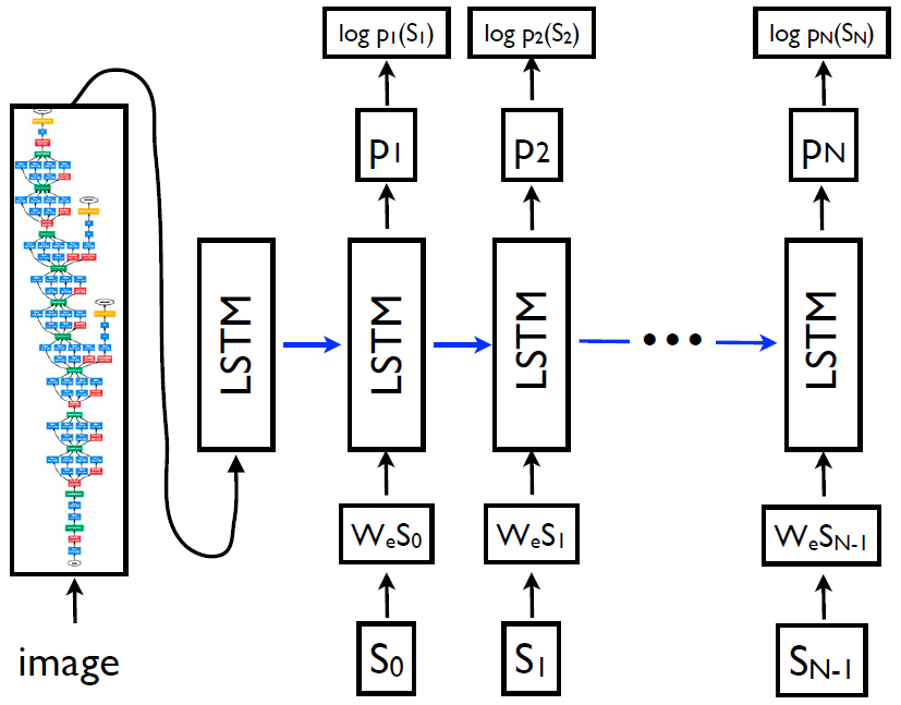
NIC

This paper presents a generative model based on a deep recurrent architecture that combines recent advances in computer vision and machine translation and that can be used to generate natural sentences describing an image. The model uses the encoder-decoder framework of machine translation, which replaces the encoder RNN by a deep convolution neural network.

It must be emphasized that:

1. The model uses a more powerful CNN in the encoder, which yields the best performance on the ILSVRC 2014 classification competition at that time.
2. To deal with vanishing and exploding gradients, LSTM was introduced in the decoder to generate sentences based on the fixed-length vector representations from CNN.
3. The image is only input once, at t = -1, to inform the LSTM about the image contents.

   We empirically verified that feeding the image at each time step as an extra input yields inferior results, as the network can explicitly exploit noise in the image and overfits more easily.

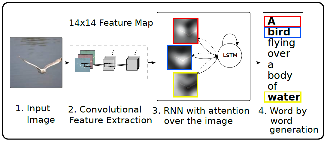
Attention-Based

One of the most curious facets of the human visual system is the presence of attention. Rather than compress an entire image into a static representation, attention allows for salient features to dynamically come to the forefront as needed. This is especially important when there is a lot of clutter in an image.

Using representations (such as those from the top layer of a convnet) that distill information in image down to the most salient objects is one effective solution that has been widely adopted in previous work. Unfortunately, this has one potential drawback of losing information which could be useful for richer, more descriptive captions.

Using more low-level representation can help preserve this information. However, working with these features necessitates a powerful mechanism to steer the model to information important to the task at hand.

This paper describes approaches to caption generation that attempt to incorporate a form of attention with two variants:

1. a “soft” deterministic attention mechanism trainable by standard back-propagation methods
2. a “hard” stochastic attention mechanism trainable by maximizing an approximate variational lower bound or equivalently by REINFORCE

The paper above introducing the attention-based model was published at ICML-2015. Since then, there has been a lot of models developed by researchers, and the state of the art was broken again and again.

If you are interested in this field, you can also click on this link, which summarizes many excellent papers in image captioning.

Now, let's begin with our implementation.

Image Captioning

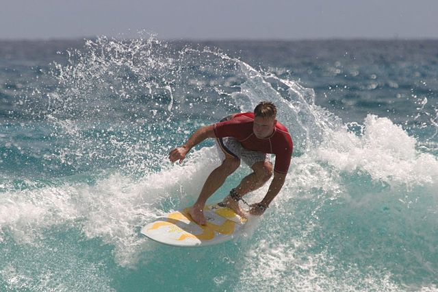
Given an image like the example below, our goal is to generate a caption such as "a surfer riding on a wave".

Image Source; License: Public Domain

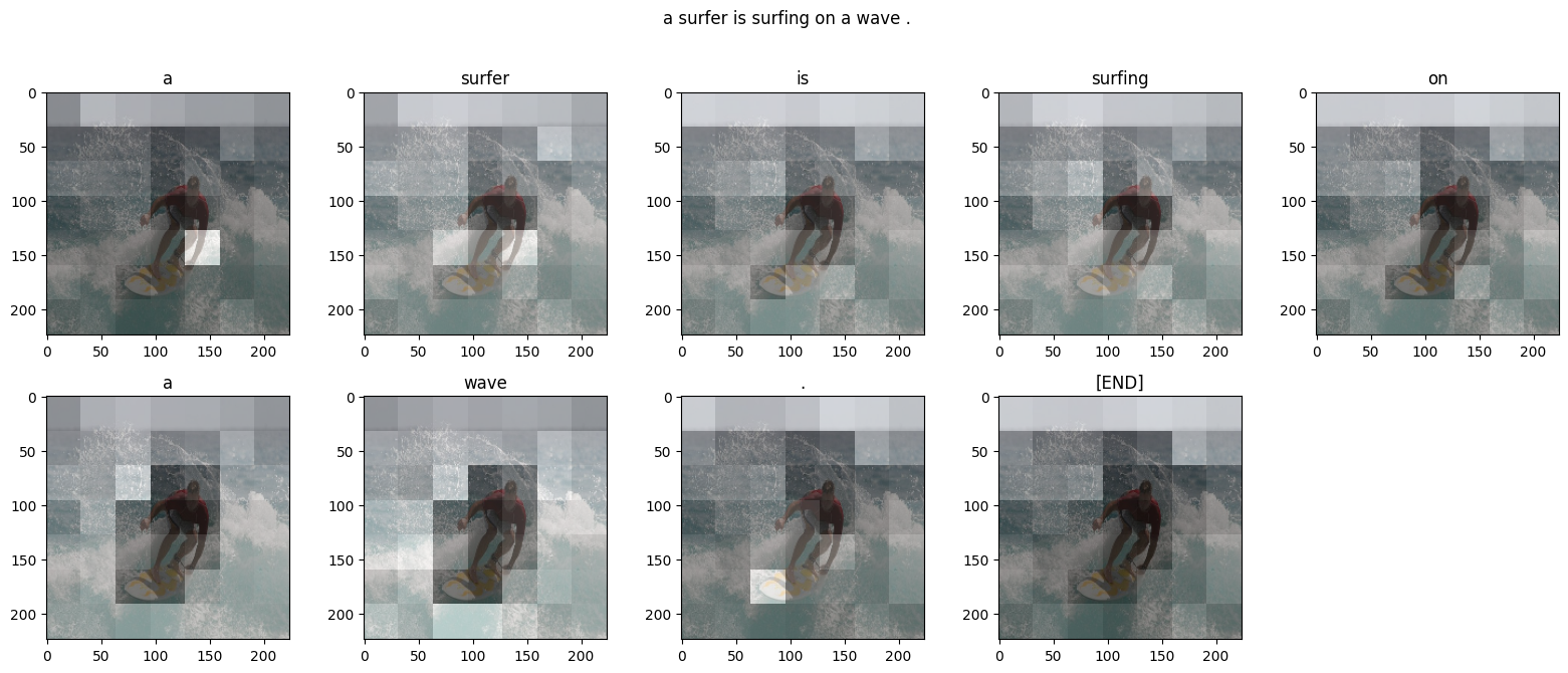
To accomplish this, you'll use an attention-based model, which enables us to see what parts of the image the model focuses on as it generates a caption.

The model architecture is similar to Show, Attend and Tell: Neural Image Caption Generation with Visual Attention.

This notebook is an end-to-end example. When you run the notebook, it downloads the MS-COCO dataset, preprocesses and caches a subset of images using Inception V3, trains an encoder-decoder model, and generates captions on new images using the trained model.

import tensorflow as tf
gpus = tf.config.experimental.list_physical_devices('GPU')
if gpus:
    try:
        # Currently, memory growth needs to be the same across GPUs
        for gpu in gpus:
            tf.config.experimental.set_memory_growth(gpu, True)
        tf.config.experimental.set_visible_devices(gpus[0], 'GPU')
        logical_gpus = tf.config.experimental.list_logical_devices('GPU')
        print(len(gpus), "Physical GPUs,", len(logical_gpus), "Logical GPUs")
    except RuntimeError as e:
        # Memory growth must be set before GPUs have been initialized
        print(e)

1 Physical GPUs, 1 Logical GPUs

# You'll generate plots of attention in order to see which parts of an image
# our model focuses on during captioning
import matplotlib.pyplot as plt

# Scikit-learn includes many helpful utilities
from sklearn.model_selection import train_test_split
from sklearn.utils import shuffle

import re
import numpy as np
import os
import time
import json
from glob import glob
from PIL import Image
import pickle

Download and prepare the MS-COCO dataset

You will use the MS-COCO dataset to train our model. The dataset contains over 82,000 images, each of which has at least 5 different caption annotations. The code below downloads and extracts the dataset automatically.

Caution: large download ahead. You'll use the training set, which is a 13GB file.

directory = './' # where you want to put the zip files and images
if not os.path.exists(directory+'captions.zip'):
    annotation_zip = tf.keras.utils.get_file( directory + 'captions.zip',
                                              cache_subdir=directory,
                                              origin = 'http://images.cocodataset.org/annotations/annotations_trainval2014.zip',
                                              extract = True)
annotation_file = directory +'annotations/captions_train2014.json'


if not os.path.exists(directory + 'train2014.zip'):
    image_zip = tf.keras.utils.get_file(directory + 'train2014.zip',
                                      cache_subdir=directory,
                                      origin = 'http://images.cocodataset.org/zips/train2014.zip',
                                      extract = True)
PATH = directory +'train2014/'

Optional: limit the size of the training set

To speed up training for this tutorial, you'll use a subset of 30,000 captions and their corresponding images to train our model. Choosing to use more data would result in improved captioning quality.

# Read the json file
with open(annotation_file, 'r') as f:
    annotations = json.load(f)

# Store captions and image names in vectors
all_captions = []
all_img_name_vector = []

for annot in annotations['annotations']:
    caption = '<start> ' + annot['caption'] + ' <end>'
    image_id = annot['image_id']
    full_coco_image_path = PATH + 'COCO_train2014_' + '%012d.jpg' % (image_id)

    all_img_name_vector.append(full_coco_image_path)
    all_captions.append(caption)

# Shuffle captions and image_names together
# Set a random state
train_captions, img_name_vector = shuffle(all_captions,
                                          all_img_name_vector,
                                          random_state=1)

# Select the first 30,000 captions from the shuffled set
num_examples = 30000
train_captions = train_captions[:num_examples]
img_name_vector = img_name_vector[:num_examples]

len(train_captions), len(all_captions) , len([name for name in os.listdir(PATH) if os.path.isfile(os.path.join(PATH, name))])

(30000, 414113, 82783)

There are tottal 82,783 images with 414,113 captions, but we only use 30,000 captions and their corresponding images to train our model.

Preprocess the images using InceptionV3

Next, you will use InceptionV3 (which is pretrained on Imagenet) to classify each image. You will extract features from the last convolutional layer.

First, you will convert the images into InceptionV3's expected format by:

• Resizing the image to 299px by 299px
• Preprocess the images using the preprocess_input method to normalize the image so that it contains pixels in the range of -1 to 1, which matches the format of the images used to train InceptionV3.

def load_image(image_path):
    img = tf.io.read_file(image_path)
    img = tf.image.decode_jpeg(img, channels=3)
    img = tf.image.resize(img, (299, 299))
    img = tf.keras.applications.inception_v3.preprocess_input(img)
    return img, image_path

Initialize InceptionV3 and load the pretrained Imagenet weights

Now you'll create a tf.keras model where the output layer is the last convolutional layer in the InceptionV3 architecture. The shape of the output of this layer is 8x8x2048. You use the last convolutional layer because you are using attention in this example. You don't perform this initialization during training because it could become a bottleneck.

• You forward each image through the network and store the resulting vector in a dictionary (image_name --> feature_vector).
• After all the images are passed through the network, you pickle the dictionary and save it to disk.

image_model = tf.keras.applications.InceptionV3(include_top=False,
                                                weights='imagenet')
new_input = image_model.input
hidden_layer = image_model.layers[-1].output

image_features_extract_model = tf.keras.Model(new_input, hidden_layer)

Caching the features extracted from InceptionV3

You will pre-process each image with InceptionV3 and cache the output to disk. Caching the output in RAM would be faster but also memory intensive, requiring 8 * 8 * 2048 floats per image. At the time of writing, this exceeds the memory limitations of Colab (currently 12GB of memory).

Performance could be improved with a more sophisticated caching strategy (for example, by sharding the images to reduce random access disk I/O), but that would require more code.

The caching will take about 10 minutes to run in Colab with a GPU. If you'd like to see a progress bar, you can:

1. install tqdm:

   !pip install -q tqdm

2. Import tqdm:

   from tqdm import tqdm

3. Change the following line:

   for img, path in image_dataset:

   to:

   for img, path in tqdm(image_dataset):

Note: the code below would take more than 12GB of memory to save the features extracted by inception_v3

from tqdm import tqdm

# Get unique images
encode_train = sorted(set(img_name_vector))

# Feel free to change batch_size according to your system configuration
image_dataset = tf.data.Dataset.from_tensor_slices(encode_train)
image_dataset = image_dataset.map(
    load_image, num_parallel_calls=tf.data.experimental.AUTOTUNE).batch(16)

for img, path in tqdm(image_dataset):
    batch_features = image_features_extract_model(img)
    batch_features = tf.reshape(batch_features,
                              (batch_features.shape[0], -1, batch_features.shape[3]))
    
    # save the preprocessed images to .npy files
    for bf, p in zip(batch_features, path):
        path_of_feature = p.numpy().decode("utf-8")
        np.save(path_of_feature, bf.numpy())

100%|██████████| 1622/1622 [06:26<00:00,  4.20it/s]

Preprocess and tokenize the captions

• First, you'll tokenize the captions (for example, by splitting on spaces). This gives us a vocabulary of all of the unique words in the data (for example, "surfing", "football", and so on).
• Next, you'll limit the vocabulary size to the top 5,000 words (to save memory). You'll replace all other words with the token "UNK" (unknown).
• You then create word-to-index and index-to-word mappings.
• Finally, you pad all sequences to be the same length as the longest one.

# Find the maximum length of any caption in our dataset
def calc_max_length(tensor):
    return max(len(t) for t in tensor)

# Choose the top 5000 words from the vocabulary
top_k = 5000
tokenizer = tf.keras.preprocessing.text.Tokenizer(num_words=top_k,
                                                  oov_token="<unk>",
                                                  filters='!"#$%&()*+.,-/:;=?@[\]^_`{|}~ ')
tokenizer.fit_on_texts(train_captions)
train_seqs = tokenizer.texts_to_sequences(train_captions)

tokenizer.word_index['<pad>'] = 0
tokenizer.index_word[0] = '<pad>'

# Create the tokenized vectors
train_seqs = tokenizer.texts_to_sequences(train_captions)

# Pad each vector to the max_length of the captions
# If you do not provide a max_length value, pad_sequences calculates it automatically
cap_vector = tf.keras.preprocessing.sequence.pad_sequences(train_seqs, padding='post')

# Calculates the max_length, which is used to store the attention weights
max_length = calc_max_length(train_seqs)

Split the data into training and testing

# Create training and validation sets using an 80-20 split
img_name_train, img_name_val, cap_train, cap_val = train_test_split(img_name_vector,
                                                                    cap_vector,
                                                                    test_size=0.2,
                                                                    random_state=0)

len(img_name_train), len(cap_train), len(img_name_val), len(cap_val)

(24000, 24000, 6000, 6000)

Create a tf.data dataset for training

Our images and captions are ready! Next, let's create a tf.data dataset to use for training our model.

# Feel free to change these parameters according to your system's configuration

BATCH_SIZE = 100
BUFFER_SIZE = 5000
embedding_dim = 256
units = 512
vocab_size = len(tokenizer.word_index) + 1
num_steps = len(img_name_train) // BATCH_SIZE
# Shape of the vector extracted from InceptionV3 is (64, 2048)
# These two variables represent that vector shape
features_shape = 2048
attention_features_shape = 64

# Load the numpy files
def map_func(img_name, cap):
    img_tensor = np.load(img_name.decode('utf-8')+'.npy')
    return img_tensor, cap

dataset = tf.data.Dataset.from_tensor_slices((img_name_train, cap_train))

# Use map to load the numpy files in parallel
dataset = dataset.map(lambda item1, item2: tf.numpy_function(
          map_func, [item1, item2], [tf.float32, tf.int32]),
          num_parallel_calls=tf.data.experimental.AUTOTUNE)

# Shuffle and batch
dataset = dataset.shuffle(BUFFER_SIZE).batch(BATCH_SIZE)
dataset = dataset.prefetch(buffer_size=tf.data.experimental.AUTOTUNE)

Model

Fun fact: the decoder below is identical to the one in the example for Neural Machine Translation with Attention.

The model architecture is inspired by the Show, Attend and Tell paper.

• In this example, you extract the features from the lower convolutional layer of InceptionV3 giving us a vector of shape (8, 8, 2048).
• You squash that to a shape of (64, 2048).
• This vector is then passed through the CNN Encoder (which consists of a single Fully connected layer).
• The RNN (here GRU) attends over the image to predict the next word.

class BahdanauAttention(tf.keras.Model):
    def __init__(self, units):
        super(BahdanauAttention, self).__init__()
        self.W1 = tf.keras.layers.Dense(units)
        self.W2 = tf.keras.layers.Dense(units)
        self.V = tf.keras.layers.Dense(1)

    def call(self, features, hidden):
        # features(CNN_encoder output) shape == (batch_size, 64, embedding_dim)

        # hidden shape == (batch_size, hidden_size)
        # hidden_with_time_axis shape == (batch_size, 1, hidden_size)
        hidden_with_time_axis = tf.expand_dims(hidden, 1)

        # score shape == (batch_size, 64, hidden_size)
        score = tf.nn.tanh(self.W1(features) + self.W2(hidden_with_time_axis))

        # attention_weights shape == (batch_size, 64, 1)
        # you get 1 at the last axis because you are applying score to self.V
        attention_weights = tf.nn.softmax(self.V(score), axis=1)

        # context_vector shape after sum == (batch_size, hidden_size)
        context_vector = attention_weights * features
        context_vector = tf.reduce_sum(context_vector, axis=1)

        return context_vector, attention_weights

class CNN_Encoder(tf.keras.Model):
    # Since you have already extracted the features and dumped it using pickle
    # This encoder passes those features through a Fully connected layer
    def __init__(self, embedding_dim):
        super(CNN_Encoder, self).__init__()
        # shape after fc == (batch_size, 64, embedding_dim)
        self.fc = tf.keras.layers.Dense(embedding_dim)

    def call(self, x):
        x = self.fc(x)
        x = tf.nn.relu(x)
        return x

class RNN_Decoder(tf.keras.Model):
    def __init__(self, embedding_dim, units, vocab_size):
        super(RNN_Decoder, self).__init__()
        self.units = units

        self.embedding = tf.keras.layers.Embedding(vocab_size, embedding_dim)
        self.gru = tf.keras.layers.GRU(self.units,
                                       return_sequences=True,
                                       return_state=True,
                                       recurrent_initializer='glorot_uniform')
        self.fc1 = tf.keras.layers.Dense(self.units)
        self.fc2 = tf.keras.layers.Dense(vocab_size)

        self.attention = BahdanauAttention(self.units)

    def call(self, x, features, hidden):
        # defining attention as a separate model
        context_vector, attention_weights = self.attention(features, hidden)

        # x shape after passing through embedding == (batch_size, 1, embedding_dim)
        x = self.embedding(x)

        # x shape after concatenation == (batch_size, 1, embedding_dim + hidden_size)
        x = tf.concat([tf.expand_dims(context_vector, 1), x], axis=-1)

        # passing the concatenated vector to the GRU
        output, state = self.gru(x)

        # shape == (batch_size, max_length, hidden_size)
        x = self.fc1(output)

        # x shape == (batch_size * max_length, hidden_size)
        x = tf.reshape(x, (-1, x.shape[2]))

        # output shape == (batch_size * max_length, vocab)
        x = self.fc2(x)

        return x, state, attention_weights

    def reset_state(self, batch_size):
        return tf.zeros((batch_size, self.units))

encoder = CNN_Encoder(embedding_dim)
decoder = RNN_Decoder(embedding_dim, units, vocab_size)

optimizer = tf.keras.optimizers.Adam()
loss_object = tf.keras.losses.SparseCategoricalCrossentropy(
    from_logits=True, reduction='none')

def loss_function(real, pred):
    mask = tf.math.logical_not(tf.math.equal(real, 0))
    loss_ = loss_object(real, pred)

    mask = tf.cast(mask, dtype=loss_.dtype)
    loss_ *= mask

    return tf.reduce_mean(loss_)

Checkpoint

checkpoint_path = "./checkpoints/train"
ckpt = tf.train.Checkpoint(encoder=encoder,
                           decoder=decoder,
                           optimizer = optimizer)
ckpt_manager = tf.train.CheckpointManager(ckpt, checkpoint_path, max_to_keep=3)

start_epoch = 0
if ckpt_manager.latest_checkpoint:
    start_epoch = int(ckpt_manager.latest_checkpoint.split('-')[-1])

Training

• You extract the features stored in the respective .npy files and then pass those features through the encoder.
• The encoder output, hidden state(initialized to 0) and the decoder input (which is the start token) is passed to the decoder.
• The decoder returns the predictions and the decoder hidden state.
• The decoder hidden state is then passed back into the model and the predictions are used to calculate the loss.
• Use teacher forcing to decide the next input to the decoder.
• Teacher forcing is the technique where the target word is passed as the next input to the decoder.
• The final step is to calculate the gradients and apply it to the optimizer and backpropagate.

# adding this in a separate cell because if you run the training cell
# many times, the loss_plot array will be reset
loss_plot = []

@tf.function
def train_step(img_tensor, target):
    loss = 0

    # initializing the hidden state for each batch
    # because the captions are not related from image to image
    hidden = decoder.reset_state(batch_size=target.shape[0])

    dec_input = tf.expand_dims([tokenizer.word_index['<start>']] * BATCH_SIZE, 1)

    with tf.GradientTape() as tape:
        features = encoder(img_tensor)

        for i in range(1, target.shape[1]):
            # passing the features through the decoder
            predictions, hidden, _ = decoder(dec_input, features, hidden)

            loss += loss_function(target[:, i], predictions)

            # using teacher forcing
            dec_input = tf.expand_dims(target[:, i], 1)

    total_loss = (loss / int(target.shape[1]))

    trainable_variables = encoder.trainable_variables + decoder.trainable_variables

    gradients = tape.gradient(loss, trainable_variables)

    optimizer.apply_gradients(zip(gradients, trainable_variables))

    return loss, total_loss

EPOCHS = 50
start = time.time()
for epoch in range(start_epoch, EPOCHS):
    
    total_loss = 0

    for (batch, (img_tensor, target)) in tqdm(enumerate(dataset), total=num_steps):
        batch_loss, t_loss = train_step(img_tensor, target)
        total_loss += t_loss

#         if batch % 100 == 0:
#             print ('Epoch {} Batch {} Loss {:.4f}'.format(
#               epoch + 1, batch, batch_loss.numpy() / int(target.shape[1])))
    # storing the epoch end loss value to plot later
    loss_plot.append(total_loss / num_steps)

    if epoch % 5 == 0:
        ckpt_manager.save()

    print ('Epoch {} Loss {:.6f}'.format(epoch + 1,
                                         total_loss/num_steps))
print ('Time taken for {} epoch {} sec\n'.format(EPOCHS, time.time() - start))

100%|██████████| 240/240 [03:00<00:00,  1.33it/s]
  0%|          | 0/240 [00:00<?, ?it/s]

Epoch 12 Loss 1.143722

100%|██████████| 240/240 [00:49<00:00,  4.88it/s]
  0%|          | 0/240 [00:00<?, ?it/s]

Epoch 13 Loss 0.873935

100%|██████████| 240/240 [00:48<00:00,  4.90it/s]
  0%|          | 0/240 [00:00<?, ?it/s]

Epoch 14 Loss 0.777324

100%|██████████| 240/240 [00:49<00:00,  4.89it/s]
  0%|          | 0/240 [00:00<?, ?it/s]

Epoch 15 Loss 0.724108

100%|██████████| 240/240 [00:48<00:00,  4.92it/s]
  0%|          | 0/240 [00:00<?, ?it/s]

Epoch 16 Loss 0.685221

100%|██████████| 240/240 [00:49<00:00,  4.87it/s]
  0%|          | 0/240 [00:00<?, ?it/s]

Epoch 17 Loss 0.652330

100%|██████████| 240/240 [00:49<00:00,  4.86it/s]
  0%|          | 0/240 [00:00<?, ?it/s]

Epoch 18 Loss 0.622322

100%|██████████| 240/240 [00:49<00:00,  4.84it/s]
  0%|          | 0/240 [00:00<?, ?it/s]

Epoch 19 Loss 0.593033

100%|██████████| 240/240 [00:50<00:00,  4.77it/s]
  0%|          | 0/240 [00:00<?, ?it/s]

Epoch 20 Loss 0.565067

100%|██████████| 240/240 [00:49<00:00,  4.86it/s]
  0%|          | 0/240 [00:00<?, ?it/s]

Epoch 21 Loss 0.536278

100%|██████████| 240/240 [00:49<00:00,  4.88it/s]
  0%|          | 0/240 [00:00<?, ?it/s]

Epoch 22 Loss 0.508094

100%|██████████| 240/240 [00:49<00:00,  4.83it/s]
  0%|          | 0/240 [00:00<?, ?it/s]

Epoch 23 Loss 0.480660

100%|██████████| 240/240 [00:50<00:00,  4.78it/s]
  0%|          | 0/240 [00:00<?, ?it/s]

Epoch 24 Loss 0.450836

100%|██████████| 240/240 [00:49<00:00,  4.81it/s]
  0%|          | 0/240 [00:00<?, ?it/s]

Epoch 25 Loss 0.424059

100%|██████████| 240/240 [00:49<00:00,  4.85it/s]
  0%|          | 0/240 [00:00<?, ?it/s]

Epoch 26 Loss 0.396979

100%|██████████| 240/240 [00:50<00:00,  4.79it/s]
  0%|          | 0/240 [00:00<?, ?it/s]

Epoch 27 Loss 0.371712

100%|██████████| 240/240 [00:49<00:00,  4.88it/s]
  0%|          | 0/240 [00:00<?, ?it/s]

Epoch 28 Loss 0.349179

100%|██████████| 240/240 [00:49<00:00,  4.84it/s]
  0%|          | 0/240 [00:00<?, ?it/s]

Epoch 29 Loss 0.321898

100%|██████████| 240/240 [00:50<00:00,  4.71it/s]
  0%|          | 0/240 [00:00<?, ?it/s]

Epoch 30 Loss 0.299658

100%|██████████| 240/240 [00:49<00:00,  4.82it/s]
  0%|          | 0/240 [00:00<?, ?it/s]

Epoch 31 Loss 0.278836

100%|██████████| 240/240 [00:50<00:00,  4.78it/s]
  0%|          | 0/240 [00:00<?, ?it/s]

Epoch 32 Loss 0.260118

100%|██████████| 240/240 [00:50<00:00,  4.79it/s]
  0%|          | 0/240 [00:00<?, ?it/s]

Epoch 33 Loss 0.241097

100%|██████████| 240/240 [00:49<00:00,  4.82it/s]
  0%|          | 0/240 [00:00<?, ?it/s]

Epoch 34 Loss 0.225345

100%|██████████| 240/240 [00:50<00:00,  4.80it/s]
  0%|          | 0/240 [00:00<?, ?it/s]

Epoch 35 Loss 0.208650

100%|██████████| 240/240 [00:50<00:00,  4.77it/s]
  0%|          | 0/240 [00:00<?, ?it/s]

Epoch 36 Loss 0.194533

100%|██████████| 240/240 [00:48<00:00,  4.91it/s]
  0%|          | 0/240 [00:00<?, ?it/s]

Epoch 37 Loss 0.181971

100%|██████████| 240/240 [00:50<00:00,  4.73it/s]
  0%|          | 0/240 [00:00<?, ?it/s]

Epoch 38 Loss 0.170026

100%|██████████| 240/240 [00:50<00:00,  4.77it/s]
  0%|          | 0/240 [00:00<?, ?it/s]

Epoch 39 Loss 0.158259

100%|██████████| 240/240 [00:50<00:00,  4.78it/s]
  0%|          | 0/240 [00:00<?, ?it/s]

Epoch 40 Loss 0.152570

100%|██████████| 240/240 [00:49<00:00,  4.81it/s]
  0%|          | 0/240 [00:00<?, ?it/s]

Epoch 41 Loss 0.140142

100%|██████████| 240/240 [00:50<00:00,  4.76it/s]
  0%|          | 0/240 [00:00<?, ?it/s]

Epoch 42 Loss 0.130752

100%|██████████| 240/240 [00:50<00:00,  4.79it/s]
  0%|          | 0/240 [00:00<?, ?it/s]

Epoch 43 Loss 0.121833

100%|██████████| 240/240 [00:49<00:00,  4.82it/s]
  0%|          | 0/240 [00:00<?, ?it/s]

Epoch 44 Loss 0.115533

100%|██████████| 240/240 [00:50<00:00,  4.77it/s]
  0%|          | 0/240 [00:00<?, ?it/s]

Epoch 45 Loss 0.109346

100%|██████████| 240/240 [00:50<00:00,  4.79it/s]
  0%|          | 0/240 [00:00<?, ?it/s]

Epoch 46 Loss 0.102974

100%|██████████| 240/240 [00:50<00:00,  4.77it/s]
  0%|          | 0/240 [00:00<?, ?it/s]

Epoch 47 Loss 0.103317

100%|██████████| 240/240 [00:50<00:00,  4.79it/s]
  0%|          | 0/240 [00:00<?, ?it/s]

Epoch 48 Loss 0.097723

100%|██████████| 240/240 [00:49<00:00,  4.86it/s]
  0%|          | 0/240 [00:00<?, ?it/s]

Epoch 49 Loss 0.095953

100%|██████████| 240/240 [00:49<00:00,  4.88it/s]

Epoch 50 Loss 0.088175
Time taken for 50 epoch 2081.1310606002808 sec

plt.plot(loss_plot)
plt.xlabel('Epochs')
plt.ylabel('Loss')
plt.title('Loss Plot')
plt.show()

Caption!

• The evaluate function is similar to the training loop, except you don't use teacher forcing here. The input to the decoder at each time step is its previous predictions along with the hidden state and the encoder output.
• Stop predicting when the model predicts the end token.
• And store the attention weights for every time step.

def evaluate(image):
    attention_plot = np.zeros((max_length, attention_features_shape))

    hidden = decoder.reset_state(batch_size=1)

    temp_input = tf.expand_dims(load_image(image)[0], 0)
    img_tensor_val = image_features_extract_model(temp_input)
    img_tensor_val = tf.reshape(img_tensor_val, (img_tensor_val.shape[0], -1, img_tensor_val.shape[3]))

    features = encoder(img_tensor_val)

    dec_input = tf.expand_dims([tokenizer.word_index['<start>']], 0)
    result = []

    for i in range(max_length):
        predictions, hidden, attention_weights = decoder(dec_input, features, hidden)

        attention_plot[i] = tf.reshape(attention_weights, (-1, )).numpy()

        predicted_id = tf.argmax(predictions[0]).numpy()
        result.append(tokenizer.index_word[predicted_id])

        if tokenizer.index_word[predicted_id] == '<end>':
            return result, attention_plot

        dec_input = tf.expand_dims([predicted_id], 0)

    attention_plot = attention_plot[:len(result), :]
    return result, attention_plot

def plot_attention(image, result, attention_plot):
    temp_image = np.array(Image.open(image))

    fig = plt.figure(figsize=(10, 10))

    len_result = len(result)
    for l in range(len_result):
        temp_att = np.resize(attention_plot[l], (8, 8))
        ax = fig.add_subplot(len_result//2, len_result//2, l+1)
        ax.set_title(result[l])
        img = ax.imshow(temp_image)
        ax.imshow(temp_att, cmap='gray', alpha=0.6, extent=img.get_extent())

    plt.tight_layout()
    plt.show()

# captions on the validation set
rid = np.random.randint(0, len(img_name_val))
image = img_name_val[rid]
real_caption = ' '.join([tokenizer.index_word[i] for i in cap_val[rid] if i not in [0]])
result, attention_plot = evaluate(image)

print ('Real Caption:', real_caption)
print ('Prediction Caption:', ' '.join(result))
plot_attention(image, result, attention_plot)
# opening the image
Image.open(img_name_val[rid])

Real Caption: <start> a young bear cub is leashed or the amusement of the crowd <end>
Prediction Caption: a group of people sitting around a hill <end>

Try it on your own images

For fun, below we've provided a method you can use to caption your own images with the model we've just trained. Keep in mind, it was trained on a relatively small amount of data, and your images may be different from the training data (so be prepared for weird results!)

image_url = 'https://tensorflow.org/images/surf.jpg'
image_extension = image_url[-4:]
image_path = tf.keras.utils.get_file('image'+image_extension,
                                     origin=image_url)

result, attention_plot = evaluate(image_path)
print ('Prediction Caption:', ' '.join(result))
plot_attention(image_path, result, attention_plot)
# opening the image
Image.open(image_path)

Prediction Caption: a man is surfing on a surfboard in the ocean <end>

Assignment

CAPTCHA (an acronym for "Completely Automated Public Turing test to tell Computers and Humans Apart") is a type of challenge–response test used in computing to determine whether or not the user is human, which is a popular tool since it prevents spam attacks and protects websites from bots.

Captcha asks you to complete the math equation like addition, subtraction, or multiplication. The equation can show up using numbers, letters, or images, therefore bots have no chances.

reCAPTCHA is a CAPTCHA-like system designed to establish that a computer user is human (normally in order to protect websites from bots) and, at the same time, assist in the digitization of books or improve machine learning (even its slogan was “Stop Spam, Read Books”).

It supports two versions. The first asks you to enter some words or digits from the image, and the second asks you to mark the checkbox “I’m not a robot”.

So, as you can see, both tools provide the same functionality increasing the security level of your websites, but the way of how it looks is different. For the more, they also have differences in their features. Let’s compare them:

CAPTCHAs of English words contain information about the words, so we can use CNN to extract it from images. As you know, RNN can capture the interdependencies between sequences, so it is perfect for generating words by RNN based on the extracted information.

In this assignment, you have to train a captcha-recognizer which can identify English words in images.

You can download the dataset here.

Description of Dataset:

1. There are 140,000 images in this dataset containing 2500 English words (3-5 character lengths) in four different fonts.
2. In all of these images, there are some noises(lines, curves and points) in different colors.

The captcha is shown in the figure below:

Requirements

1. You can use any model architectures (or any code above) you want, as long as accomplishing the goal.
2. You should train your own model architecture. In other words, except the feature extractor part, do not load the model or any pre-trained weights directly from other sources.
   • You can use pretrained inception_v3 as feature extractor; however, it's not recommended since inception is pretrained on ImageNet, where the image pattern is quite different to English words.
3. You should use the first 100,000 images as training data, the next 20,000 as validation data, and the rest (final 20,000) as testing data.
   • spec_train_val.txt contains the labels of only first 120,000 images.
4. Only if the whole word matches exactly does it count as correct.
5. You need to predict the answer to the testing data and write them in a file.
6. Your testing accuracy should be at least 90% in validation set.

Hint

In image caption, we expect RNN would output one word at each step, so we use tf.keras.preprocessing.text.Tokenizer to create a mapping relationship between words and indices on a word-by-word basis.

However, in captcha, we expect RNN would output one character at each step. Therefore, before calling Tokenizer, you need to preprocess the training data in a certain form (refer to the text description in the 'Preprocess and tokenize the captions' section), so that we can correctly establish the mapping relationship between character and index by the Tokenizer.

Notification:

• Submit on eeclass your code file (Lab12-2_{student id}.ipynb), and your answer file (Lab12-2_{student id}.txt).
  • Answer file please follow the format as spec_train_val.txt.
• Give a brief report for every parts you have done.
• The deadline will be 2024/11/21 00:00.